如果你也在 怎样代写宏观经济学Macroeconomics 这个学科遇到相关的难题,请随时右上角联系我们的24/7代写客服。宏观经济学Macroeconomics对国家或地区经济整体行为的研究。它关注的是对整个经济事件的理解,如商品和服务的生产总量、失业水平和价格的一般行为。宏观经济学关注的是经济体的表现–经济产出、通货膨胀、利率和外汇兑换率以及国际收支的变化。减贫、社会公平和可持续增长只有在健全的货币和财政政策下才能实现。
宏观经济学Macroeconomics(来自希腊语前缀makro-,意思是 “大 “+经济学)是经济学的一个分支,处理整个经济体的表现、结构、行为和决策。例如,使用利率、税收和政府支出来调节经济的增长和稳定。这包括区域、国家和全球经济。根据经济学家Emi Nakamura和Jón Steinsson在2018年的评估,经济 “关于不同宏观经济政策的后果的证据仍然非常不完善,并受到严重批评。宏观经济学家研究的主题包括GDP(国内生产总值)、失业(包括失业率)、国民收入、价格指数、产出、消费、通货膨胀、储蓄、投资、能源、国际贸易和国际金融。
statistics-lab™ 为您的留学生涯保驾护航 在代写宏观经济学Macroeconomics方面已经树立了自己的口碑, 保证靠谱, 高质且原创的统计Statistics代写服务。我们的专家在代写宏观经济学Macroeconomics代写方面经验极为丰富,各种代写宏观经济学Macroeconomics相关的作业也就用不着说。
经济代写|宏观经济学代写Macroeconomics代考|Proportion of Income Spent on the Good
The price elasticity of demand for a good also has implications for total revenue. Total revenue (TR) is the amount sellers receive for a good or service. Total revenue is simply the price of the good $(P)$ times the quantity of the good sold $(Q): T R=P \times Q$. The elasticity of demand will help to predict how changes in the price will impact total revenue earned by the producer for selling the good. Let’s see how this works.
In Exhibit 1 , we see that when the demand is price elastic $\left(E_{\mathrm{D}}>1\right)$, total revenues will rise as the price declines, because the percentage increase in the quantity demanded is greater than the percentage reduction in price. For example, if the price of a good is cut in half (say from $\$ 10$ to $\$ 5$ ) and the quantity demanded more than doubles (say from 40 to 100 ), total revenue will rise from $\$ 400(\$ 10 \times 40=\$ 400)$ to $\$ 500(\$ 5 \times 100=\$ 500)$. Equivalently, if the price rises from $\$ 5$ to $\$ 10$ and the quantity demanded falls from 100 to 40 units, then total revenue will fall from $\$ 500$ to $\$ 400$. As this example illustrates, if the demand curve is relatively elastic, total revenue will vary inversely with a price change.
You can see from the following what happens to total revenue when demand is price elastic. (Note: The size of the price and quantity arrows represents the size of the percentage changes.)
When Demand Is Price Elastic
$$
\downarrow T R=\uparrow P \times \downarrow Q
$$
or
$$
\uparrow T R=\downarrow P \times \uparrow Q
$$
On the other hand, if demand for a good is relatively inelastic $\left(E_{\mathrm{D}}<1\right)$, the total revenue will be lower at lower prices than at higher prices because a given price reduction will be accompanied by a proportionately smaller increase in quantity demanded. For example, as shown in Exhibit 2, if the price of a good is cut (say from $\$ 10$ to $\$ 5$ ) and the quantity demanded less than doubles (say it increases from 30 to 40 ), then total revenue will fall from $\$ 300(\$ 10 \times 30=\$ 300)$ to $\$ 200(\$ 5 \times 40=\$ 200)$. Equivalently, if the price increases from $\$ 5$ to $\$ 10$ and the quantity demanded falls from 40 to 30 , total revenue will increase from $\$ 200$ to $\$ 300$. That is, if the demand curve is inelastic, total revenue will vary directly with a price change.
When Demand Is Price Inelastic
$$
\begin{aligned}
\uparrow T R= & \uparrow P \times \downarrow Q \
& \text { or } \
\downarrow T R= & \downarrow P \times \uparrow Q
\end{aligned}
$$
or
In this case, the “net” effect on total revenue is reversed but easy to see. (Again, the size of the price and quantity arrows represents the size of the percentage changes.)
经济代写|宏观经济学代写Macroeconomics代考|Price Elasticity Changes along a Linear Demand Curve
As already shown (Section 6.1, Exhibit 1), the slopes of demand curves can be used to estimate their relative elasticities of demand: The steeper one demand curve is relative to another, the more inelastic it is relative to the other. However, except for the extreme cases of perfectly elastic and perfectly inelastic curves, great care must be taken when trying to estimate the degree of elasticity of one demand curve from its slope. In fact, as we will soon see, a straight-line demand curve with a constant slope will change elasticity continuously as you move up or down it. It is because the slope is the ratio of changes in the two variables (price and quantity) while the elasticity is the ratio of percentage changes in the two variables.
We can easily demonstrate that the elasticity of demand varies along a linear demand curve by using what we already know about the interrelationship between price and total revenue.
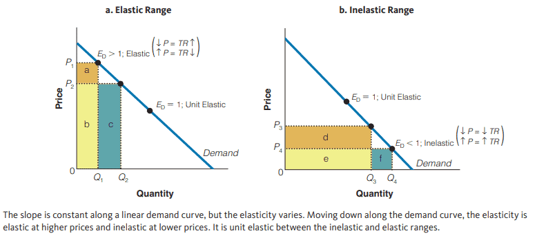
Exhibit 4 shows a linear (constant slope) demand curve. In Exhibit 4(a), we see that when the price falls on the upper half of the demand curve from $P_1$ to $P_2$, and quantity demanded increases from $Q_1$ to $Q_2$, total revenue increases. That is, the new area of total revenue $($ area $b+c$ ) is larger than the old area of total revenue (area $a+b)$. It is also true that if price increased in this region (from $P_2$ to $P_1$ ), total revenue would fall because $\mathrm{b}+\mathrm{c}$ is greater than $\mathrm{a}+\mathrm{b}$.
In this region of the demand curve, then, there is a negative relationship between price and total revenue. As we discussed earlier, this is characteristic of an elastic demand curve $\left(E_{\mathrm{D}}>1\right)$.
Exhibit 4(b) illustrates what happens to total revenue on the lower half of the same demand curve. When the price falls from $P_3$ to $P_4$ and the quantity demanded increases from $Q_3$ to $Q_4$, total revenue actually decreases because the new area of total revenue (area $\mathrm{e}+\mathrm{f}$ ) is less than the old area of total revenue (area $\mathrm{d}+\mathrm{e}$ ). Likewise, it is clear that an increase in price from $P_4$ to $P_3$ would increase total revenue. In this case, there is a positive relationship between price and total revenue, which, as we discussed, is characteristic of an inelastic demand curve $\left(E_{\mathrm{D}}<1\right)$. Together, parts (a) and (b) of Exhibit 4 illustrate that, although the slope remains constant, the elasticity of a linear demand curve changes along the length of the curve-from relatively elastic at higher price ranges to relatively inelastic at lower price ranges.

宏观经济学代考
经济代写|宏观经济学代写Macroeconomics代考|Proportion of Income Spent on the Good
商品需求的价格弹性也会影响总收入。总收益(TR)是卖方从商品或服务中获得的金额。总收入就是商品的价格$(P)$乘以商品的销售量$(Q): T R=P \times Q$。需求弹性将有助于预测价格的变化将如何影响生产者销售商品所获得的总收入。让我们看看它是如何工作的。
在表1中,我们看到,当需求具有价格弹性$\left(E_{\mathrm{D}}>1\right)$时,总收益将随着价格下降而上升,因为需求量增加的百分比大于价格下降的百分比。例如,如果一种商品的价格减半(比如从$\$ 10$降至$\$ 5$),而需求量增加一倍以上(比如从40降至100),总收入将从$\$ 400(\$ 10 \times 40=\$ 400)$上升至$\$ 500(\$ 5 \times 100=\$ 500)$。同样地,如果价格从$\$ 5$上升到$\$ 10$,需求量从100下降到40,那么总收益将从$\$ 500$下降到$\$ 400$。如本例所示,如果需求曲线是相对弹性的,总收入将与价格变化成反比。
从下图可以看出,当需求具有价格弹性时,总收入的变化情况。(注:价格和数量箭头的大小代表百分比变化的大小。)
当需求具有价格弹性时
$$
\downarrow T R=\uparrow P \times \downarrow Q
$$
或
$$
\uparrow T R=\downarrow P \times \uparrow Q
$$
另一方面,如果对一种商品的需求相对缺乏弹性$\left(E_{\mathrm{D}}<1\right)$,则总收益在价格较低时将低于价格较高时,因为给定的价格降低将伴随着按比例较小的需求量增加。例如,如图2所示,如果一种商品的价格降低(比如从$\$ 10$降至$\$ 5$),而需求量增加一倍以下(比如从30增加到40),那么总收入将从$\$ 300(\$ 10 \times 30=\$ 300)$降至$\$ 200(\$ 5 \times 40=\$ 200)$。同样,如果价格从$\$ 5$上升到$\$ 10$,需求量从40下降到30,总收益将从$\$ 200$上升到$\$ 300$。也就是说,如果需求曲线是非弹性的,总收入将直接随价格变化而变化。
当需求价格无弹性时
$$
\begin{aligned}
\uparrow T R= & \uparrow P \times \downarrow Q \
& \text { or } \
\downarrow T R= & \downarrow P \times \uparrow Q
\end{aligned}
$$
或
在这种情况下,对总收入的“净”影响是相反的,但很容易看到。(同样,价格和数量箭头的大小表示百分比变化的大小。)
经济代写|宏观经济学代写Macroeconomics代考|Price Elasticity Changes along a Linear Demand Curve
如前所述(第6.1节,表1),需求曲线的斜率可以用来估计需求的相对弹性:一条需求曲线相对于另一条需求曲线越陡峭,它相对于另一条需求曲线的弹性就越小。然而,除了完全弹性曲线和完全非弹性曲线的极端情况外,在试图从一条需求曲线的斜率估计其弹性程度时,必须非常小心。事实上,我们很快就会看到,斜率为常数的直线需求曲线会随着上下移动而不断改变弹性。这是因为斜率是两个变量(价格和数量)变化的比率,而弹性是两个变量变化百分比的比率。
通过使用我们已经知道的价格和总收入之间的相互关系,我们可以很容易地证明需求弹性沿着线性需求曲线变化。
图4显示了一条线性(斜率恒定)需求曲线。在图4(a)中,我们看到,当价格在需求曲线的上半部分从$P_1$下降到$P_2$时,需求量从$Q_1$增加到$Q_2$,总收入增加。也就是说,总收入的新区域$(区域$b+c$)大于总收入的旧区域$(区域$a+b)$。同样,如果该区域的价格上涨(从$P_2$到$P_1$),总收益将下降,因为$\ mathm {b}+\ mathm {c}$大于$\ mathm {a}+\ mathm {b}$。
因此,在需求曲线的这个区域,价格和总收入之间存在负相关关系。正如我们前面所讨论的,这是弹性需求曲线$\left(E_{\ mathm {D}}>1\right)$的特征。
图4(b)展示了同一需求曲线下半部分的总收入。当价格从$P_3$下降到$P_4$,需求量从$Q_3$增加到$Q_4$时,总收入实际上减少了,因为总收入的新区域($\ mathm {e}+\ mathm {f}$)小于总收入的旧区域($\ mathm {d}+\ mathm {e}$)。同样,很明显,价格从$P_4$增加到$P_3$会增加总收入。在这种情况下,价格和总收入之间存在正关系,正如我们所讨论的,这是非弹性需求曲线$\left(E_{\ mathm {D}}<1\right)$的特征。图4的(a)和(b)部分共同说明,尽管斜率保持不变,但线性需求曲线的弹性沿着曲线的长度变化——从较高价格区间的相对弹性到较低价格区间的相对无弹性。

统计代写请认准statistics-lab™. statistics-lab™为您的留学生涯保驾护航。
金融工程代写
金融工程是使用数学技术来解决金融问题。金融工程使用计算机科学、统计学、经济学和应用数学领域的工具和知识来解决当前的金融问题,以及设计新的和创新的金融产品。
非参数统计代写
非参数统计指的是一种统计方法,其中不假设数据来自于由少数参数决定的规定模型;这种模型的例子包括正态分布模型和线性回归模型。
广义线性模型代考
广义线性模型(GLM)归属统计学领域,是一种应用灵活的线性回归模型。该模型允许因变量的偏差分布有除了正态分布之外的其它分布。
术语 广义线性模型(GLM)通常是指给定连续和/或分类预测因素的连续响应变量的常规线性回归模型。它包括多元线性回归,以及方差分析和方差分析(仅含固定效应)。
有限元方法代写
有限元方法(FEM)是一种流行的方法,用于数值解决工程和数学建模中出现的微分方程。典型的问题领域包括结构分析、传热、流体流动、质量运输和电磁势等传统领域。
有限元是一种通用的数值方法,用于解决两个或三个空间变量的偏微分方程(即一些边界值问题)。为了解决一个问题,有限元将一个大系统细分为更小、更简单的部分,称为有限元。这是通过在空间维度上的特定空间离散化来实现的,它是通过构建对象的网格来实现的:用于求解的数值域,它有有限数量的点。边界值问题的有限元方法表述最终导致一个代数方程组。该方法在域上对未知函数进行逼近。[1] 然后将模拟这些有限元的简单方程组合成一个更大的方程系统,以模拟整个问题。然后,有限元通过变化微积分使相关的误差函数最小化来逼近一个解决方案。
tatistics-lab作为专业的留学生服务机构,多年来已为美国、英国、加拿大、澳洲等留学热门地的学生提供专业的学术服务,包括但不限于Essay代写,Assignment代写,Dissertation代写,Report代写,小组作业代写,Proposal代写,Paper代写,Presentation代写,计算机作业代写,论文修改和润色,网课代做,exam代考等等。写作范围涵盖高中,本科,研究生等海外留学全阶段,辐射金融,经济学,会计学,审计学,管理学等全球99%专业科目。写作团队既有专业英语母语作者,也有海外名校硕博留学生,每位写作老师都拥有过硬的语言能力,专业的学科背景和学术写作经验。我们承诺100%原创,100%专业,100%准时,100%满意。
随机分析代写
随机微积分是数学的一个分支,对随机过程进行操作。它允许为随机过程的积分定义一个关于随机过程的一致的积分理论。这个领域是由日本数学家伊藤清在第二次世界大战期间创建并开始的。
时间序列分析代写
随机过程,是依赖于参数的一组随机变量的全体,参数通常是时间。 随机变量是随机现象的数量表现,其时间序列是一组按照时间发生先后顺序进行排列的数据点序列。通常一组时间序列的时间间隔为一恒定值(如1秒,5分钟,12小时,7天,1年),因此时间序列可以作为离散时间数据进行分析处理。研究时间序列数据的意义在于现实中,往往需要研究某个事物其随时间发展变化的规律。这就需要通过研究该事物过去发展的历史记录,以得到其自身发展的规律。
回归分析代写
多元回归分析渐进(Multiple Regression Analysis Asymptotics)属于计量经济学领域,主要是一种数学上的统计分析方法,可以分析复杂情况下各影响因素的数学关系,在自然科学、社会和经济学等多个领域内应用广泛。
MATLAB代写
MATLAB 是一种用于技术计算的高性能语言。它将计算、可视化和编程集成在一个易于使用的环境中,其中问题和解决方案以熟悉的数学符号表示。典型用途包括:数学和计算算法开发建模、仿真和原型制作数据分析、探索和可视化科学和工程图形应用程序开发,包括图形用户界面构建MATLAB 是一个交互式系统,其基本数据元素是一个不需要维度的数组。这使您可以解决许多技术计算问题,尤其是那些具有矩阵和向量公式的问题,而只需用 C 或 Fortran 等标量非交互式语言编写程序所需的时间的一小部分。MATLAB 名称代表矩阵实验室。MATLAB 最初的编写目的是提供对由 LINPACK 和 EISPACK 项目开发的矩阵软件的轻松访问,这两个项目共同代表了矩阵计算软件的最新技术。MATLAB 经过多年的发展,得到了许多用户的投入。在大学环境中,它是数学、工程和科学入门和高级课程的标准教学工具。在工业领域,MATLAB 是高效研究、开发和分析的首选工具。MATLAB 具有一系列称为工具箱的特定于应用程序的解决方案。对于大多数 MATLAB 用户来说非常重要,工具箱允许您学习和应用专业技术。工具箱是 MATLAB 函数(M 文件)的综合集合,可扩展 MATLAB 环境以解决特定类别的问题。可用工具箱的领域包括信号处理、控制系统、神经网络、模糊逻辑、小波、仿真等。