数学代写|凸优化作业代写Convex Optimization代考|Proximal Algorithm, Bundle Methods, and Tikhonov Regularization
数学代写|凸优化作业代写Convex Optimization代考|Proximal Algorithm, Bundle Methods, and Tikhonov Regularization
The proximal algorithm, briefly discussed in Section 2.1.4, aims to minimize a closed proper convex function $f: \Re^n \mapsto(-\infty, \infty)$, and is given by $$ x_{k+1} \in \arg \min _{x \in \Re^n}\left{f(x)+\frac{1}{2 c_k}\left|x-x_k\right|^2\right} $$ [cf. Eq. (2.25)], where $x_0$ is an arbitrary starting point and $c_k$ is a positive scalar parameter. As the parameter $c_k$ tends to $\infty$, the quadratic regularization term becomes insignificant and the proximal minimization (2.55) approximates more closely the minimization of $f$, hence the connection of the proximal algorithm with the approximation approach.
We will discuss the proximal algorithm in much more detail in Chapter 5 , including dual and polyhedral approximation versions. Among others, we will show that when $f$ is the dual function of the constrained optimization problem (2.50), the proximal algorithm, via Fenchel duality, becomes equivalent to the multiplier iteration of the augmented Lagrangian method [cf. Eq. (2.54)]. Since any closed proper convex function can be viewed as the dual function of an appropriate convex constrained optimization problem, it follows that the proximal algorithm (2.55) is essentially equivalent to the augmented Lagrangian method: the two algorithms are dual sides of the same coin.
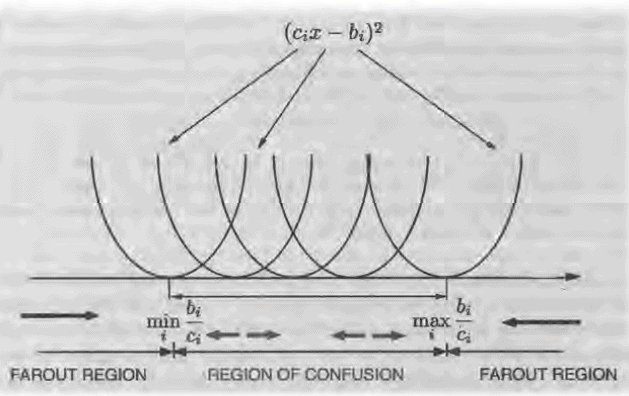
There are also variants of the proximal algorithm where $f$ in Eq. (2.55) is approximated by a polyhedral or other function. One possibility is bundle methods, which involve a combination of the proximal and polyhedral approximation ideas. The motivation here is to simplify the proximal minimization subproblem (2.25), replacing it for example with a quadratic programming problem. Some of these methods may be viewed as regularized versions of Dantzig-Wolfe decomposition (see Section 4.3). Another approximation approach that bears similarity to the proximal algorithm is Tikhonov regularization, which approximates the minimization of $f$ with the minimization $$ x_{k+1} \in \arg \min _{x \in \Re^n}\left{f(x)+\frac{1}{2 c_k}|x|^2\right} . $$
数学代写|凸优化作业代写Convex Optimization代考|Alternating Direction Method of Multipliers
The proximal algorithm embodies fundamental ideas that lead to a variety of other interesting methods. In particular, when properly generalized (see Section 5.1.4), it contains as a special case the alternating direction method of multipliers (ADMM for short), a method that resembles the augmented Lagrangian method, but is well-suited for some important classes of problems with special structure.
The starting point for the ADMM is the minimization problem of the Fenchel duality context: $$ \begin{aligned} & \text { minimize } f_1(x)+f_2(A x) \ & \text { subject to } x \in \Re^n, \end{aligned} $$ where $A$ is an $m \times n$ matrix, $f_1: \Re^n \mapsto(-\infty, \infty]$ and $f_2: \Re^m \mapsto(-\infty, \infty]$ are closed proper convex functions. We convert this problem to the equivalent constrained minimization problem $$ \begin{array}{ll} \operatorname{minimize} & f_1(x)+f_2(z) \ \text { subject to } & x \in \Re^n, z \in \Re^m, \quad A x=z, \end{array} $$ and we introduce its augmented Lagrangian function $$ L_c(x, z, \lambda)=f_1(x)+f_2(z)+\lambda^{\prime}(A x-z)+\frac{c}{2}|A x-z|^2, $$ where $c$ is a positive parameter. The ADMM, given the current iterates $\left(x_k, z_k, \lambda_k\right) \in \Re^n \times \Re^m \times \Re^m$, generates a new iterate $\left(x_{k+1}, z_{k+1}, \lambda_{k+1}\right)$ by first minimizing the augmented Lagrangian with respect to $x$, then with respect to $z$, and finally performing a multiplier update: $$ \begin{gathered} x_{k+1} \in \arg \min {x \in \Re^n} L_c\left(x, z_k, \lambda_k\right), \ z{k+1} \in \arg \min {z \in \Re^m} L_c\left(x{k+1}, z, \lambda_k\right), \ \lambda_{k+1}=\lambda_k+c\left(A x_{k+1}-z_{k+1}\right) . \end{gathered} $$
数学代写|凸优化作业代写Convex Optimization代考|Proximal Algorithm, Bundle Methods, and Tikhonov Regularization
Incremental subgradient methods are related to methods that aim to minimize an expected value $$ f(x)=E{F(x, w)} $$ where $w$ is a random variable, and $F(\cdot, w): \Re^n \mapsto \Re$ is a convex function for each possible value of $w$. The stochastic subgradient method for minimizing $f$ over a closed convex set $X$ is given by $$ x_{k+1}=P_X\left(x_k-\alpha_k g\left(x_k, w_k\right)\right) $$
where $w_k$ is a sample of $w$ and $g\left(x_k, w_k\right)$ is a subgradient of $F\left(\cdot, w_k\right)$ at $x_k$. This method has a rich theory and a long history, particularly for the case where $F(\cdot, w)$ is differentiable for each value of $w$ (for representative references, see [PoT73], [Lju77], [KuC78], [TBA86], [Pol87], [BeT89a], [BeT96], [Pf196], [LBB98], [BeT00], [KuY03], [Bot05], [BeL07], [Mey07], [Bor08], [BBG09], [Ben09], [NJL09], [Bot10], [BaM11], [DHS11], [ShZ12], [FrG13], [NSW14]). It is strongly related to the classical algorithmic field of stochastic approximation; see the books [KuC78], [BeT96], [KuY03], $[$ Spa03], [Mey07], [Bor08], [BPP13].
If we view the expected value cost $E{F(x, w)}$ as a weighted sum of cost function components, we see that the stochastic subgradient method (2.40) is related to the incremental subgradient method $$ x_{k+1}=P_X\left(x_k-\alpha_k g_{i, k}\right) $$ for minimizing a finite sum $\sum_{i=1}^m f_i$, when randomization is used for component selection [cf. Eq. (2.31)]. An important difference is that the former method involves sequential sampling of cost components $F(x, w)$ from an infinite population under some statistical assumptions, while in the latter the set of cost components $f_i$ is predetermined and finite. However, it is possible to view the incremental subgradient method $(2.41)$, with uniform randomized selection of the component function $f_i$ (i.e., with $i_k$ chosen to be any one of the indexes $1, \ldots, m$, with equal probability $1 / m$, and independently of preceding choices), as a stochastic subgradient method.
数学代写|凸优化作业代写Convex Optimization代考|Incremental Newton Methods
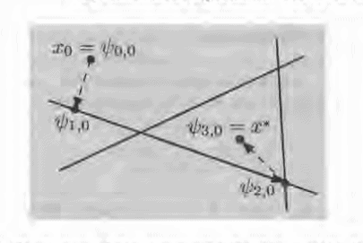
We will now consider an incremental version of Newton’s method for unconstrained minimization of an additive cost function of the form $$ f(x)=\sum_{i=1}^m f_i(x) $$ where the functions $f_i: \Re^n \mapsto \Re$ are convex and twice continuously differentiable. Consider the quadratic approximation $\tilde{f}i$ of a function $f_i$ at a vector $\psi \in \Re^n$, i.e., the second order Taylor expansion of $f_i$ at $\psi$ : $$ \tilde{f}_i(x ; \psi)=\nabla f_i(\psi)^{\prime}(x-\psi)+\frac{1}{2}(x-\psi)^{\prime} \nabla^2 f_i(\psi)(x-\psi), \quad \forall x, \psi \in \Re^n . $$ Similar to Newton’s method, which minimizes a quadratic approximation at the current point of the cost function [cf. Eq. (2.14)], the incremental form of Newton’s method minimizes a sum of quadratic approximations of components. Similar to the incremental gradient method, we view an iteration as a cycle of $m$ subiterations, each involving a single additional component $f_i$, and its gradient and Hessian at the current point within the cycle. In particular, if $x_k$ is the vector obtained after $k$ cycles, the vector $x{k+1}$ obtained after one more cycle is $$ x_{k+1}=\psi_{m, k} $$ where starting with $\psi_{0, k}=x_k$, we obtain $\psi_{m, k}$ after the $m$ steps $$ \psi_{i, k} \in \arg \min {x \in \Re^n} \sum{\ell=1}^i \tilde{f}{\ell}\left(x ; \psi{\ell-1, k}\right), \quad i=1, \ldots, m $$
数学代写|现代代数代写Modern Algebra代考|Mignotte’s factor bound and a modular gcd algorithm in Z[x]
数学代写|现代代数代写Modern Algebra代考|Mignotte’s factor bound and a modular gcd algorithm in Z[x]
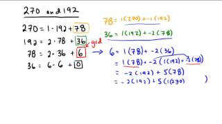
In order to adapt Algorithm 6.28 to $\mathbb{Z}[x]$, we need an a priori bound on the coefficient size of $h$. Over $F[y]$, the bound $$ \operatorname{deg}_y h \leq \operatorname{deg}_y f $$ is trivial and quite sufficient. Over $\mathbb{Z}$, we could use the subresultant bound of Theorem 6.52 below, but we now derive a much better bound. It actually depends only on one argument of the gcd, say $f$, and is valid for all factors of $f$. We will use this again for the factorization of $f$ in Chapter 15 .
We extend the 2-norm to a complex polynomial $f=\sum_{0 \leq i \leq n} f_i x^i \in \mathbb{C}[x]$ by $|f|_2=\left(\sum_{0 \leq i \leq n}\left|f_i\right|^2\right)^{1 / 2} \in \mathbb{R}$, where $|a|=(a \cdot \bar{a})^{1 / 2} \in \mathbb{R}$ is the norm of $a \in \mathbb{C}$ and $\bar{a}$ is the complex conjugate of $a$. We will derive a bound for the norm of factors of $f$ in terms of $|f|_2$, that is, a bound $B \in \mathbb{R}$ such that any factor $h \in \mathbb{Z}[x]$ of $f$ satisfies $|h|_2 \leq B$. One might hope that we can take $B=|f|_2$, but this is not the case. For example, let $f=x^n-1$ and $h=\Phi_n \in \mathbb{Z}[x]$ be the $n$th cyclotomic polynomial (Section 14.10). Thus $\Phi_n$ divides $x^n-1$, and the direct analog of (8) would say that each coefficient of $\Phi_n$ is at most 1 in absolute value, but for example $\Phi_{105}$, of degree 48 , contains the term $-2 x^7$. In fact, the coefficients of $\Phi_n$ are unbounded in absolute value if $n \longrightarrow \infty$, and hence this is also true for $|h|_2$. Worse yet, for infinitely many integers $n, \Phi_n$ has a very large coefficient, namely larger than $\exp (\exp (\ln 2 \cdot \ln n / \ln \ln n))$, where $\ln$ is the logarithm in base $e$; such a coefficient has word length somewhat less than $n$. It is not obvious how to control the coefficients of factors at all, and it is not surprising that we have to work a little bit to establish a good bound.
We have seen in Section 5.5 that the small primes modular approach for computing the determinant is computationally superior to the big prime scheme. The reason that we have discussed big prime modular gcd algorithms at all in the preceding sections is that they are easier and the main idea is more clearly visible than for their small prime variants that we will present now. In practice, we strongly recommend the use of the latter. We start with the algorithm for $F[x, y]$ since it is simpler to describe and analyze than the corresponding algorithm for $\mathbb{Z}[x]$. AlgORITHM 6.36 Modular bivariate ged: small primes version. Input: Primitive polynomials $f, g \in F[x, y]=R[x]$ with $\operatorname{deg}_x f=n \geq \operatorname{deg}_x g \geq 1$ and $\operatorname{deg}_y f, \operatorname{deg}_y g \leq d$, where $R=F[y]$ for a field $F$ with at least $(4 n+2) d$ elements. Output: $h=\operatorname{gcd}(f, g) \in R[x]$.
$b \longleftarrow \operatorname{gcd}\left(\operatorname{lc}_x(f), \operatorname{lc}_x(g)\right), \quad l \longleftarrow d+1+\operatorname{deg}_y b$
repeat
choose a set $S \subseteq F$ of $2 l$ evaluation points
$S \longleftarrow{u \in S: b(u) \neq 0}$ for each $u \in S$ call the Euclidean Algorithm 3.14 over $F$ to compute the monic $v_u=\operatorname{gcd}(f(x, u), g(x, u)) \in F[x]$
$e \longleftarrow \min \left{\operatorname{deg} v_u: u \in S\right}, \quad S \longleftarrow\left{u \in S: \operatorname{deg} v_u=e\right}$ if $# S \geq l$ then remove $# S-l$ elements from $S$ else goto 3
compute by interpolation each coefficient in $F[y]$ of the polynomials $w, f^, g^ \in R[x]$ of degrees in $y$ less than $l$ such that $$ w(x, u)=b(u) v_u $$
$$ f^(x, u) w(x, u)=b(u) f(x, u), \quad g^(x, u) w(x, u)=b(u) g(x, u) $$ for all $u \in S$
until $\operatorname{deg}_y\left(f^* w\right)=\operatorname{deg}_y(b f)$ and $\operatorname{deg}_y\left(g^* w\right)=\operatorname{deg}_y(b g)$
return $\mathrm{pp}_x(w)$
数学代写|现代代数代写Modern Algebra代考|Mignotte’s factor bound and a modular gcd algorithm in Z[x]
数学代写|现代代数代写Modern Algebra代考|Mignotte’s factor bound and a modular gcd algorithm in Z[x]
为了使算法6.28适应$\mathbb{Z}[x]$,我们需要对$h$的系数大小有一个先验的界。除以$F[y]$,边界 $$ \operatorname{deg}_y h \leq \operatorname{deg}_y f $$ 是微不足道的,而且是足够的。在$\mathbb{Z}$上,我们可以使用下面定理6.52的次结界,但我们现在推导出一个更好的界。它实际上只依赖于gcd的一个参数,比如$f$,并且对$f$的所有因素都有效。我们将在第15章中再次使用它来分解$f$。
We discuss another one of the numerous applications of the Chinese Remainder Theorem for polynomials. It will be put to use in Chapter 22 .
Let $F$ be a field, $f_1, \ldots, f_r \in F[x]$ nonconstant monic and pairwise coprime polynomials, $e_1, \ldots, e_r \in \mathbb{N}$ positive integers, and $f=f_1^{e_1} \cdots f_r^{e_r}$. (We will see in Part III how to factor polynomials over finite fields and over $\mathbb{Q}$ into irreducible factors, but here we do not assume irreducibility of the $f_i$.) For another polynomial $g \in F[x]$ of degree less than $n=\operatorname{deg} f$, the partial fraction decomposition of the rational function $g / f \in F(x)$ with respect to the given factorization of the denominator $f$ is $$ \frac{g}{f}=\frac{g_{1,1}}{f_1}+\cdots+\frac{g_{1, e_1}}{f_1^{e_1}}+\cdots+\frac{g_{r, 1}}{f_r}+\cdots+\frac{g_{r, e_r}}{f_r^{e_r}}, $$ with $g_{i j} \in F[x]$ of smaller degree than $f_i$, for all $i, j$. If all $f_i$ are linear polynomials, then the $g_{i j}$ are just constants.
EXAMPLE 5.28. Let $F=\mathbb{Q}, f=x^4-x^2$, and $g=x^3+4 x^2-x-2$. The partial fraction decomposition of $g / f$ with respect to the factorization $f=x^2(x-1)(x+1)$ of $f$ into linear polynomials is $$ \frac{x^3+4 x^2-x-2}{x^4-x^2}=\frac{1}{x}+\frac{2}{x^2}+\frac{1}{x-1}+\frac{-1}{x+1} $$ The following questions pose themselves: Does a decomposition as in (31) always exist uniquely, and how can we compute it? The next lemma is a first step towards an answer.
数学代写|现代代数代写Modern Algebra代考|Coefficient growth in the Euclidean Algorithm
Let $F$ be a field, and $f, g \in F[x]$ with $\operatorname{deg} f=n \geq \operatorname{deg} g=m \geq 0$. We fix the notation from Section 3.4 of the results of the Extended Euclidean Algorithm for $f$ and $g$ : $$ \begin{aligned} & \rho_0 r_0=f \ & \rho_0 s_0=1 \text {, } \ & \rho_0 t_0=0, \ & \rho_1 r_1=g \ & \rho_1 s_1=0 \text {, } \ & \rho_1 t_1=1 \text {, } \ & \rho_2 r_2=r_0-q_1 r_1 \text {, } \ & \rho_2 s_2=s_0-q_1 s_1 \text {, } \ & \rho_2 t_2=t_0-q_1 t_1 \text {, } \ & \vdots \ & \vdots \ & \text { : } \ & \rho_{i+1} r_{i+1}=r_{i-1}-q_i r_i, \quad \rho_{i+1} s_{i+1}=s_{i-1}-q_i s_i, \quad \rho_{i+1} t_{i+1}=t_{i-1}-q_i t_i, \ & \vdots \ & 0=r_{\ell-1}-q_{\ell} r_{\ell}, \ & \vdots \ & \text { : } \ & s_{\ell+1}=s_{\ell-1}-q_{\ell} s_{\ell}, \ & t_{\ell+1}=t_{\ell-1}-q_{\ell} t_{\ell}, \ & \end{aligned} $$
with $\operatorname{deg} r_{i+1}<\operatorname{deg} r_i$ for all $i \geq 1$. Thus $r_{i-1}=q_i r_i+\rho_{i+1} r_{i+1}$ is the division of $r_{i-1}$ by $r_i$ with remainder $\rho_{i+1} r_{i+1}$; the leading coefficient $\rho_{i+1}$ serves to have a normalized remainder $r_{i+1}$. A basic invariant is $r_i=s_i f+t_i g$. We define the degree sequence $\left(n_0, n_1, \ldots, n_{\ell}\right)$ by $n_i=\operatorname{deg} r_i$ for all $i$. Then $$ n=n_0 \geq n_1>n_2 \cdots>n_{\ell} \geq 0 . $$ It is convenient to set $\rho_{\ell+1}=1, r_{\ell+1}=0$, and $n_{\ell+1}=-\infty$. The number of arithmetic operations in $F$ performed by the (Extended) Euclidean Algorithm for $f$ and $g$ is $O(n m)$ (Theorem 3.16).
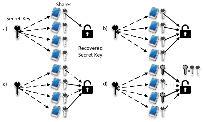
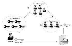
A neat application of interpolation, which we mentioned in Section 1.3 but which will not be used later, is secret sharing: you want to give to $n$ players a shared secret, so that together they can discover it, but no proper subset of the players can. To achieve this, you identify possible secrets with elements of the finite field $\mathbb{F}_p=\mathbb{Z} /\langle p\rangle$ for an appropriate $p$. Some bank cards for Automatic Teller Machine access have as their secret PIN codes four-digit decimal numbers. For such a secret, you choose a prime $p$ just bigger than 10000 , say $p=10007$. Then you choose $2 n-1$ random elements $f_1, \ldots, f_{n-1}, u_0, \ldots, u_{n-1} \in \mathbb{F}p$ uniformly and independently with all $u_i$ nonzero, call your secret $f_0$, set $f=f{n-1} x^{n-1}+\cdots+f_1 x+f_0 \in$ $\mathbb{F}_p[x]$, and give to player number $i$ the value $f\left(u_i\right) \in \mathbb{F}_p$. (If $u_i=u_j$ for some $i \neq j$, you have to make a new random choice; this is unlikely to happen if $n \ll \sqrt{p}$.) Then together they can determine the (unique) interpolation polynomial $f$ of degree less than $n$, and thus $f_0$. But if any smaller number of them, say $n-1$, get together, then the possible interpolation polynomials consistent with this partial knowledge are such that each value in $\mathbb{F}_p$ of $f_0$ is equally likely: they have no information on $f_0$ (Exercise 5.14).
We can extend this scheme to the situation where $k \leq n$ and each subset of $k$ players are able to recover the secret, but no set of fewer than $k$ players can. This is achieved by randomly and independently choosing $n+k-1$ elements $u_0, \ldots, u_{n-1}, f_1, \ldots, f_{k-1} \in \mathbb{F}p$ and giving $f\left(u_i\right)$ to player $i$, where $f=f{k-1} x^{k-1}+$ $\cdots+f_1 x+f_0 \in \mathbb{F}_p[x]$ and $f_0 \in \mathbb{F}_p$ is the secret as above. Again, it is required that $u_i \neq u_j$ if $i \neq j$. Since $f$ is uniquely determined by its values at $k$ points, each subset of $k$ out of the $n$ players can calculate $f$ and thus the secret $f_0$, but fewer than $k$ players together have no information on $f_0$.
数学代写|现代代数代写Modern Algebra代考|The Chinese Remainder Algorithm
Suppose that $f \in \mathbb{N}$ has two decimal digits and has remainder 2 on division by 11 and 7 on division by 13 . Does this uniquely define $f$, and if so, is there a better way to find it than to check all values between 0 and 99 ? We will see in this section that the answer to both questions is positive. For this section, $R$ is a Euclidean domain, and we fix the following notation: $m_0, \ldots, m_{r-1} \in R$ are pairwise coprime, so that $\operatorname{gcd}\left(m_i, m_j\right)=1$ for $0 \leq i<j<r$, and $m=m_0 \cdots m_{r-1}$. Thus $m=\operatorname{lcm}\left(m_0, \ldots, m_{r-1}\right)$. For $0 \leq i<r$, we have the canonical ring homomorphism $$ \begin{aligned} \pi_i: R & \longrightarrow R /\left\langle m_i\right\rangle, \ f & \longmapsto f \bmod m_i . \end{aligned} $$ Combining these for all $i$, we get the ring homomorphism $$ \begin{aligned} & \chi=\pi_0 \times \cdots \times \pi_{r-1}: R \longrightarrow R /\left\langle m_0\right\rangle \times \ldots \times R /\left\langle m_{r-1}\right\rangle, \ & f \longmapsto\left(f \bmod m_0, \ldots, f \bmod m_{r-1}\right) \text {. } \ & \end{aligned} $$ For our example above, we have $R=\mathbb{Z}, r=2, m_0=11, m_1=13, m=143$, and $$ \chi(f)=(f \bmod 11, f \bmod 13)=(2 \bmod 11,7 \bmod 13) \in \mathbb{Z}{11} \times \mathbb{Z}{13} . $$ The following statement provides, in somewhat abstract terminology, the theoretical basis for many of our algorithms.
Let us return once more to König’s duality theorem for bipartite graphs, Theorem 2.1.1. If we orient every edge of $G$ from $A$ to $B$, the theorem tells us how many disjoint directed paths we need in order to cover all the vertices of $G$ : every directed path has length 0 or 1 , and clearly the number of paths in such a ‘path cover’ is smallest when it contains as many paths of length 1 as possible – in other words, when it contains a maximum-cardinality matching.
In this section we put the above question more generally: how many paths in a given directed graph will suffice to cover its entire vertex set? Of course, this could be asked just as well for undirected graphs. As it turns out, however, the result we shall prove is rather more trivial in the undirected case (exercise), and the directed case will also have an interesting corollary.
A directed path is a directed graph $P \neq \emptyset$ with distinct vertices $x_0, \ldots, x_k$ and edges $e_0, \ldots, e_{k-1}$ such that $e_i$ is an edge directed from $x_i$ to $x_{i+1}$, for all $i<k$. In this section, path will always mean ‘directed path’. The vertex $x_k$ above is the last vertex of the path $P$, and when $\mathcal{P}$ is a set of paths we write $\operatorname{ter}(\mathcal{P})$ for the set of their last vertices. A path cover of a directed graph $G$ is a set of disjoint paths in $G$ which together contain all the vertices of $G$.
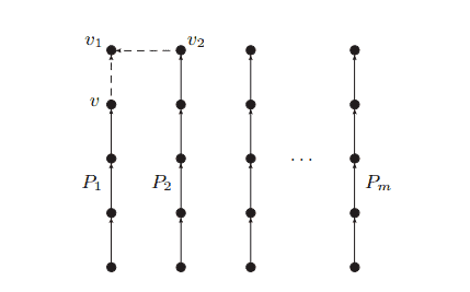
Theorem 2.5.1. (Gallai \& Milgram 1960) Every directed graph $G$ has a path cover $\mathcal{P}$ and an independent set $\left{v_P \mid P \in \mathcal{P}\right}$ of vertices such that $v_P \in P$ for every $P \in \mathcal{P}$.
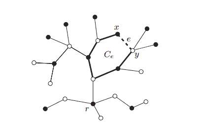
Proof. We prove by induction on $|G|$ that for every path cover $\mathcal{P}=$ $\left{P_1, \ldots, P_m\right}$ of $G$ with $\operatorname{ter}(\mathcal{P})$ minimal there is a set $\left{v_P \mid P \in \mathcal{P}\right}$ as claimed. For each $i$, let $v_i$ denote the last vertex of $P_i$.
If $\operatorname{ter}(\mathcal{P})=\left{v_1, \ldots, v_m\right}$ is independent there is nothing more to show, so we assume that $G$ has an edge from $v_2$ to $v_1$. Since $P_2 v_2 v_1$ is again a path, the minimality of $\operatorname{ter}(\mathcal{P})$ implies that $v_1$ is not the only vertex of $P_1$; let $v$ be the vertex preceding $v_1$ on $P_1$. Then $\mathcal{P}^{\prime}:=$ $\left{P_1 v, P_2, \ldots, P_m\right}$ is a path cover of $G^{\prime}:=G-v_1$ (Fig. 2.5.1). Clearly, any independent set of representatives for $\mathcal{P}^{\prime}$ in $G^{\prime}$ will also work for $\mathcal{P}$ in $G$, so all we have to check is that we may apply the induction hypothesis to $\mathcal{P}^{\prime}$. It thus remains to show that $\operatorname{ter}\left(\mathcal{P}^{\prime}\right)=\left{v, v_2, \ldots, v_m\right}$ is minimal among the sets of last vertices of path covers of $G^{\prime}$.
数学代写|图论作业代写Graph Theory代考|2-Connected graphs and subgraphs
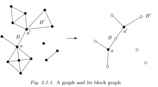
A maximal connected subgraph without a cutvertex is called a block. Thus, every block of a graph $G$ is either a maximal 2-connected subgraph, or a bridge (with its ends), or an isolated vertex. Conversely, every such subgraph is a block. By their maximality, different blocks of $G$ overlap in at most one vertex, which is then a cutvertex of $G$. Hence, every edge of $G$ lies in a unique block, and $G$ is the union of its blocks. Cycles and bonds, too, are confined to a single block:
(i) The cycles of $G$ are precisely the cycles of its blocks. (ii) The bonds of $G$ are precisely the minimal cuts of its blocks. Proof. (i) Any cycle in $G$ is a connected subgraph without a cutvertex, and hence lies in some maximal such subgraph. By definition, this is a block of $G$. (ii) Consider any cut in $G$. Let $x y$ be one of its edges, and $B$ the block containing it. By the maximality of $B$ in the definition of a block, $G$ contains no $B$-path. Hence every $x-y$ path of $G$ lies in $B$, so those edges of our cut that lie in $B$ separate $x$ from $y$ even in $G$. Assertion (ii) follows easily by repeated application of this argument.
In a sense, blocks are the 2-connected analogues of components, the maximal connected subgraphs of a graph. While the structure of $G$ is determined fully by that of its components, however, it is not captured completely by the structure of its blocks: since the blocks need not be disjoint, the way they intersect defines another structure, giving a coarse picture of $G$ as if viewed from a distance.
The following proposition describes this coarse structure of $G$ as formed by its blocks. Let $A$ denote the set of cutvertices of $G$, and $\mathcal{B}$ the set of its blocks. We then have a natural bipartite graph on $A \cup \mathcal{B}$ formed by the edges $a B$ with $a \in B$. This block graph of $G$ is shown in Figure 3.1.1.
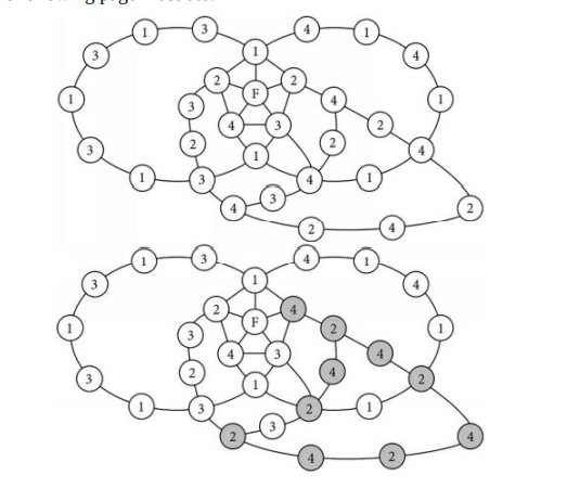
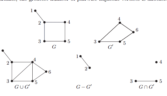
The graphs above are incomplete. These figures only show a vertex with degree four (vertex E), its nearest neighbors (A, B, C, and D), and segments of A-C Kempe chains. The entire graphs would also contain several other vertices (especially, more colored the same as B or D) and enough edges to be MPG’s. The left figure has A connected to $C$ in a single section of an A-C Kempe chain (meaning that the vertices of this chain are colored the same as A and C). The left figure shows that this A-C Kempe chain prevents B from connecting to $\mathrm{D}$ with a single section of a B-D Kempe chain. The middle figure has A and C in separate sections of A-C Kempe chains. In this case, B could connect to D with a single section of a B-D Kempe chain. However, since the A and C of the vertex with degree four lie on separate sections, the color of C’s chain can be reversed so that in the vertex with degree four, C is effectively recolored to match A’s color, as shown in the right figure. Similarly, D’s section could be reversed in the left figure so that D is effectively recolored to match B’s color.
Kempe also attempted to demonstrate that vertices with degree five are fourcolorable in his attempt to prove the four-color theorem [Ref. 2], but his argument for vertices with degree five was shown by Heawood in 1890 to be insufficient [Ref. 3]. Let’s explore what happens if we attempt to apply our reasoning for vertices with degree four to a vertex with degree five.
数学代写|图论作业代写Graph Theory代考|The previous diagrams
The previous diagrams show that when the two color reversals are performed one at a time in the crossed-chain graph, the first color reversal may break the other chain, allowing the second color reversal to affect the colors of one of F’s neighbors. When we performed the $2-4$ reversal to change B from 2 to 4 , this broke the 1-4 chain. When we then performed the 2-3 reversal to change E from 3, this caused C to change from 3 to 2 . As a result, F remains connected to four different colors; this wasn’t reversed to three as expected. Unfortunately, you can’t perform both reversals “at the same time” for the following reason. Let’s attempt to perform both reversals “at the same time.” In this crossed-chain diagram, when we swap 2 and 4 on B’s side of the 1-3 chain, one of the 4’s in the 1-4 chain may change into a 2, and when we swap 2 and 3 on E’s side of the 1-4 chain, one of the 3’s in the 1-3 chain may change into a 2 . This is shown in the following figure: one 2 in each chain is shaded gray. Recall that these figures are incomplete; they focus on one vertex (F), its neighbors (A thru E), and Kempe chains. Other vertices and edges are not shown.
Note how one of the 3’s changed into 2 on the left. This can happen when we reverse $\mathrm{C}$ and $\mathrm{E}$ (which were originally 3 and 2 ) on E’s side of the 1-4 chain. Note also how one of the 4’s changed into 2 on the right. This can happen when we reverse B and D (which were originally 2 and 4) outside of the 1-3 chain. Now we see where a problem can occur when attempting to swap the colors of two chains at the same time. If these two 2’s happen to be connected by an edge like the dashed edge shown above, if we perform the double reversal at the same time, this causes two vertices of the same color to share an edge, which isn’t allowed. We’ll revisit Kempe’s strategy for coloring a vertex with degree five in Chapter $25 .$
数学代写|图论作业代写Graph Theory代考| The shading of one section of the B-R
在上图中,顶点和是四度,因为它连接到其他四个顶点。Kempe 表明顶点 A、B、C 和 D 不能被强制为四种不同的颜色,这样顶点 E 总是可以被着色而不会违反四色定理,无论 MPG 的其余部分看起来如何上一页显示的部分。
A 和 C 或者是 AC Kempe 链的同一部分的一部分,或者它们各自位于 AC Kempe 链的不同部分。(如果一种和C例如,是红色和黄色的,则 AC 链是红黄色链。) – 如果一种和C每个位于 AC Kempe 链的不同部分,其中一个部分的颜色可以反转,这有效地重新着色 C 以匹配 A 的颜色。如果 A 和 C 是 AC Kempe 链的同一部分的一部分,则 B 和 D每个都必须位于 BD Kempe 链的不同部分,因为 AC Kempe 链将阻止任何 BD Kempe 链从 B 到达 D。(如果乙和D是蓝色和绿色,例如,那么一种BD Kempe 链是蓝绿色链。)在这种情况下,由于 B 和 D 分别位于 BD Kempe 链的不同部分,因此 BD Kempe 链的其中一个部分的颜色可以反转,这有效地重新着色 D 以匹配 B颜色。– 因此,可以使 C 与 A 具有相同的颜色或使 D 具有与 A 相同的颜色乙通过反转 Kempe 链的分离部分。
上面的图表是不完整的。这些图只显示了一个四阶顶点(顶点 E)、它的最近邻居(A、B、C 和 D),以及 AC Kempe 链的片段。整个图还将包含几个其他顶点(特别是与 B 或 D 相同的颜色)和足够多的边以成为 MPG。左图有 A 连接到C在 AC Kempe 链的单个部分中(意味着该链的顶点颜色与 A 和 C 相同)。左图显示此 AC Kempe 链阻止 B 连接到DBD Kempe 链条的一个部分。中间的数字在 AC Kempe 链的不同部分有 A 和 C。在这种情况下,B 可以通过 BD Kempe 链的单个部分连接到 D。但是,由于四阶顶点的 A 和 C 位于不同的部分,因此可以反转 C 链的颜色,以便在四阶顶点中,C 有效地重新着色以匹配 A 的颜色,如右图所示. 类似地,可以在左图中反转 D 的部分,以便有效地重新着色 D 以匹配 B 的颜色。
Let $G=(V, E)$ be a graph with $n$ vertices and $m$ edges, say $V=$ $\left{v_1, \ldots, v_n\right}$ and $E=\left{e_1, \ldots, e_m\right}$. The vertex space $\mathcal{V}(G)$ of $G$ is the vector space over the 2-element field $\mathbb{F}_2={0,1}$ of all functions $V \rightarrow \mathbb{F}_2$. Every element of $\mathcal{V}(G)$ corresponds naturally to a subset of $V$, the set of those vertices to which it assigns a 1 , and every subset of $V$ is uniquely represented in $\mathcal{V}(G)$ by its indicator function. We may thus think of $\mathcal{V}(G)$ as the power set of $V$ made into a vector space: the sum $U+U^{\prime}$ of two vertex sets $U, U^{\prime} \subseteq V$ is their symmetric difference (why?), and $U=-U$ for all $U \subseteq V$. The zero in $\mathcal{V}(G)$, viewed in this way, is the empty (vertex) set $\emptyset$. Since $\left{\left{v_1\right}, \ldots,\left{v_n\right}\right}$ is a basis of $\mathcal{V}(G)$, its standard basis, we have $\operatorname{dim} \mathcal{V}(G)=n$.
In the same way as above, the functions $E \rightarrow \mathbb{F}_2$ form the edge space $\mathcal{E}(G)$ of $G$ : its elements are the subsets of $E$, vector addition amounts to symmetric difference, $\emptyset \subseteq E$ is the zero, and $F=-F$ for all $F \subseteq E$. As before, $\left{\left{e_1\right}, \ldots,\left{e_m\right}\right}$ is the standard basis of $\mathcal{E}(G)$, and $\operatorname{dim} \mathcal{E}(G)=m$.
Since the edges of a graph carry its essential structure, we shall mostly be concerned with the edge space. Given two edge sets $F, F^{\prime} \in$ $\mathcal{E}(G)$ and their coefficients $\lambda_1, \ldots, \lambda_m$ and $\lambda_1^{\prime}, \ldots, \lambda_m^{\prime}$ with respect to the standard basis, we write $$ \left\langle F, F^{\prime}\right\rangle:=\lambda_1 \lambda_1^{\prime}+\ldots+\lambda_m \lambda_m^{\prime} \in \mathbb{F}_2 $$ Note that $\left\langle F, F^{\prime}\right\rangle=0$ may hold even when $F=F^{\prime} \neq \emptyset$ : indeed, $\left\langle F, F^{\prime}\right\rangle=0$ if and only if $F$ and $F^{\prime}$ have an even number of edges in common. Given a subspace $\mathcal{F}$ of $\mathcal{E}(G)$, we write $$ \mathcal{F}^{\perp}:={D \in \mathcal{E}(G) \mid\langle F, D\rangle=0 \text { for all } F \in \mathcal{F}} $$ This is again a subspace of $\mathcal{E}(G)$ (the space of all vectors solving a certain set of linear equations-which?), and we have $$ \operatorname{dim} \mathcal{F}+\operatorname{dim} \mathcal{F}^{\perp}=m $$
数学代写|图论作业代写Graph Theory代考|Other notions of graphs
For completeness, we now mention a few other notions of graphs which feature less frequently or not at all in this book.
A hypergraph is a pair $(V, E)$ of disjoint sets, where the elements of $E$ are non-empty subsets (of any cardinality) of $V$. Thus, graphs are special hypergraphs.
A directed graph (or digraph) is a pair $(V, E)$ of disjoint sets (of vertices and edges) together with two maps init: $E \rightarrow V$ and ter: $E \rightarrow V$ assigning to every edge $e$ an initial vertex $\operatorname{init}(e)$ and a terminal vertex ter $(e)$. The edge $e$ is said to be directed from $\operatorname{init}(e)$ to ter $(e)$. Note that a directed graph may have several edges between the same two vertices $x, y$. Such edges are called multiple edges; if they have the same direction (say from $x$ to $y$ ), they are parallel. If init $(e)=\operatorname{ter}(e)$, the edge $e$ is called a $\operatorname{loop}$.
A directed graph $D$ is an orientation of an (undirected) graph $G$ if $V(D)=V(G)$ and $E(D)=E(G)$, and if ${\operatorname{init}(e)$, ter $(e)}={x, y}$ for every edge $e=x y$. Intuitively, such an oriented graph arises from an undirected graph simply by directing every edge from one of its ends to the other. Put differently, oriented graphs are directed graphs without loops or multiple edges.
A multigraph is a pair $(V, E)$ of disjoint sets (of vertices and edges) together with a map $E \rightarrow V \cup[V]^2$ assigning to every edge either one or two vertices, its ends. Thus, multigraphs too can have loops and multiple edges: we may think of a multigraph as a directed graph whose edge directions have been ‘forgotten’. To express that $x$ and $y$ are the ends of an edge $e$ we still write $e=x y$, though this no longer determines $e$ uniquely.
有向图$D$是一个(无向)图$G$的方向,如果$V(D)=V(G)$和$E(D)=E(G)$,如果${\operatorname{init}(e)$, ter $(e)}={x, y}$对于每条边$e=x y$。直观地说,这种有向图是由无向图产生的,只要把每条边从它的一端指向另一端。换句话说,有向图是没有环路或多条边的有向图。
多图是一对$(V, E)$不相交的集合(顶点和边)和一个映射$E \rightarrow V \cup[V]^2$,每个边分配一个或两个顶点,即它的端点。因此,多图也可以有环路和多条边:我们可以认为多图是一个边缘方向被“遗忘”的有向图。为了表示$x$和$y$是边的两端$e$,我们仍然写$e=x y$,尽管这不再唯一地决定$e$。
The graphs above are incomplete. These figures only show a vertex with degree four (vertex E), its nearest neighbors (A, B, C, and D), and segments of A-C Kempe chains. The entire graphs would also contain several other vertices (especially, more colored the same as B or D) and enough edges to be MPG’s. The left figure has A connected to $C$ in a single section of an A-C Kempe chain (meaning that the vertices of this chain are colored the same as A and C). The left figure shows that this A-C Kempe chain prevents B from connecting to $\mathrm{D}$ with a single section of a B-D Kempe chain. The middle figure has A and C in separate sections of A-C Kempe chains. In this case, B could connect to D with a single section of a B-D Kempe chain. However, since the A and C of the vertex with degree four lie on separate sections, the color of C’s chain can be reversed so that in the vertex with degree four, C is effectively recolored to match A’s color, as shown in the right figure. Similarly, D’s section could be reversed in the left figure so that D is effectively recolored to match B’s color.
Kempe also attempted to demonstrate that vertices with degree five are fourcolorable in his attempt to prove the four-color theorem [Ref. 2], but his argument for vertices with degree five was shown by Heawood in 1890 to be insufficient [Ref. 3]. Let’s explore what happens if we attempt to apply our reasoning for vertices with degree four to a vertex with degree five.
数学代写|图论作业代写Graph Theory代考|The previous diagrams
The previous diagrams show that when the two color reversals are performed one at a time in the crossed-chain graph, the first color reversal may break the other chain, allowing the second color reversal to affect the colors of one of F’s neighbors. When we performed the $2-4$ reversal to change B from 2 to 4 , this broke the 1-4 chain. When we then performed the 2-3 reversal to change E from 3, this caused C to change from 3 to 2 . As a result, F remains connected to four different colors; this wasn’t reversed to three as expected. Unfortunately, you can’t perform both reversals “at the same time” for the following reason. Let’s attempt to perform both reversals “at the same time.” In this crossed-chain diagram, when we swap 2 and 4 on B’s side of the 1-3 chain, one of the 4’s in the 1-4 chain may change into a 2, and when we swap 2 and 3 on E’s side of the 1-4 chain, one of the 3’s in the 1-3 chain may change into a 2 . This is shown in the following figure: one 2 in each chain is shaded gray. Recall that these figures are incomplete; they focus on one vertex (F), its neighbors (A thru E), and Kempe chains. Other vertices and edges are not shown.
Note how one of the 3’s changed into 2 on the left. This can happen when we reverse $\mathrm{C}$ and $\mathrm{E}$ (which were originally 3 and 2 ) on E’s side of the 1-4 chain. Note also how one of the 4’s changed into 2 on the right. This can happen when we reverse B and D (which were originally 2 and 4) outside of the 1-3 chain. Now we see where a problem can occur when attempting to swap the colors of two chains at the same time. If these two 2’s happen to be connected by an edge like the dashed edge shown above, if we perform the double reversal at the same time, this causes two vertices of the same color to share an edge, which isn’t allowed. We’ll revisit Kempe’s strategy for coloring a vertex with degree five in Chapter $25 .$
数学代写|图论作业代写Graph Theory代考| The shading of one section of the B-R
在上图中,顶点和是四度,因为它连接到其他四个顶点。Kempe 表明顶点 A、B、C 和 D 不能被强制为四种不同的颜色,这样顶点 E 总是可以被着色而不会违反四色定理,无论 MPG 的其余部分看起来如何上一页显示的部分。
A 和 C 或者是 AC Kempe 链的同一部分的一部分,或者它们各自位于 AC Kempe 链的不同部分。(如果一种和C例如,是红色和黄色的,则 AC 链是红黄色链。) – 如果一种和C每个位于 AC Kempe 链的不同部分,其中一个部分的颜色可以反转,这有效地重新着色 C 以匹配 A 的颜色。如果 A 和 C 是 AC Kempe 链的同一部分的一部分,则 B 和 D每个都必须位于 BD Kempe 链的不同部分,因为 AC Kempe 链将阻止任何 BD Kempe 链从 B 到达 D。(如果乙和D是蓝色和绿色,例如,那么一种BD Kempe 链是蓝绿色链。)在这种情况下,由于 B 和 D 分别位于 BD Kempe 链的不同部分,因此 BD Kempe 链的其中一个部分的颜色可以反转,这有效地重新着色 D 以匹配 B颜色。– 因此,可以使 C 与 A 具有相同的颜色或使 D 具有与 A 相同的颜色乙通过反转 Kempe 链的分离部分。
上面的图表是不完整的。这些图只显示了一个四阶顶点(顶点 E)、它的最近邻居(A、B、C 和 D),以及 AC Kempe 链的片段。整个图还将包含几个其他顶点(特别是与 B 或 D 相同的颜色)和足够多的边以成为 MPG。左图有 A 连接到C在 AC Kempe 链的单个部分中(意味着该链的顶点颜色与 A 和 C 相同)。左图显示此 AC Kempe 链阻止 B 连接到DBD Kempe 链条的一个部分。中间的数字在 AC Kempe 链的不同部分有 A 和 C。在这种情况下,B 可以通过 BD Kempe 链的单个部分连接到 D。但是,由于四阶顶点的 A 和 C 位于不同的部分,因此可以反转 C 链的颜色,以便在四阶顶点中,C 有效地重新着色以匹配 A 的颜色,如右图所示. 类似地,可以在左图中反转 D 的部分,以便有效地重新着色 D 以匹配 B 的颜色。
A graph is a pair $G=(V, E)$ of sets such that $E \subseteq[V]^2$; thus, the elements of $E$ are 2-element subsets of $V$. To avoid notational ambiguities, we shall always assume tacitly that $V \cap E=\emptyset$. The elements of $V$ are the vertices (or nodes, or points) of the graph $G$, the elements of $E$ are its edges (or lines). The usual way to picture a graph is by drawing a dot for each vertex and joining two of these dots by a line if the corresponding two vertices form an edge. Just how these dots and lines are drawn is considered irrelevant: all that matters is the information of which pairs of vertices form an edge and which do not.
A graph with vertex set $V$ is said to be a graph on $V$. The vertex set of a graph $G$ is referred to as $V(G)$, its edge set as $E(G)$. These conventions are independent of any actual names of these two sets: the vertex set $W$ of a graph $H=(W, F)$ is still referred to as $V(H)$, not as $W(H)$. We shall not always distinguish strictly between a graph and its vertex or edge set. For example, we may speak of a vertex $v \in G$ (rather than $v \in V(G)$ ), an edge $e \in G$, and so on.
The number of vertices of a graph $G$ is its order, written as $|G|$; its number of edges is denoted by $|G|$. Graphs are finite, infinite, countable and so on according to their order. Except in Chapter 8, our graphs will be finite unless otherwise stated.
For the empty graph $(\emptyset, \emptyset)$ we simply write $\emptyset$. A graph of order 0 or 1 is called trivial. Sometimes, e.g. to start an induction, trivial graphs can be useful; at other times they form silly counterexamples and become a nuisance. To avoid cluttering the text with non-triviality conditions, we shall mostly treat the trivial graphs, and particularly the empty graph $\emptyset$, with generous disregard.
A vertex $v$ is incident with an edge $e$ if $v \in e$; then $e$ is an edge at $v$. The two vertices incident with an edge are its endvertices or ends, and an edge joins its ends. An edge ${x, y}$ is usually written as $x y$ (or $y x$ ). If $x \in X$ and $y \in Y$, then $x y$ is an $X-Y$ edge. The set of all $X-Y$ edges in a set $E$ is denoted by $E(X, Y)$; instead of $E({x}, Y)$ and $E(X,{y})$ we simply write $E(x, Y)$ and $E(X, y)$. The set of all the edges in $E$ at a vertex $v$ is denoted by $E(v)$.
数学代写|图论作业代写Graph Theory代考|The degree of a vertex
Let $G=(V, E)$ be a (non-empty) graph. The set of neighbours of a vertex $v$ in $G$ is denoted by $N_G(v)$, or briefly by $N(v) .^1$ More generally for $U \subseteq V$, the neighbours in $V \backslash U$ of vertices in $U$ are called neighbours of $U$; their set is denoted by $N(U)$.
The degree (or valency) $d_G(v)=d(v)$ of a vertex $v$ is the number $|E(v)|$ of edges at $v$; by our definition of a graph,,$^2$ this is equal to the number of neighbours of $v$. A vertex of degree 0 is isolated. The number $\delta(G):=\min {d(v) \mid v \in V}$ is the minimum degree of $G$, the number $\Delta(G):=\max {d(v) \mid v \in V}$ its maximum degree. If all the vertices of $G$ have the same degree $k$, then $G$ is $k$-regular, or simply regular. A 3 -regular graph is called cubic. The number $$ d(G):=\frac{1}{|V|} \sum_{v \in V} d(v) $$ is the average degree of $G$. Clearly, $$ \delta(G) \leqslant d(G) \leqslant \Delta(G) $$ The average degree quantifies globally what is measured locally by the vertex degrees: the number of edges of $G$ per vertex. Sometimes it will be convenient to express this ratio directly, as $\varepsilon(G):=|E| /|V|$.
The quantities $d$ and $\varepsilon$ are, of course, intimately related. Indeed, if we sum up all the vertex degrees in $G$, we count every edge exactly twice: once from each of its ends. Thus $$ |E|=\frac{1}{2} \sum_{v \in V} d(v)=\frac{1}{2} d(G) \cdot|V|, $$ and therefore $$ \varepsilon(G)=\frac{1}{2} d(G) $$
The graphs above are incomplete. These figures only show a vertex with degree four (vertex E), its nearest neighbors (A, B, C, and D), and segments of A-C Kempe chains. The entire graphs would also contain several other vertices (especially, more colored the same as B or D) and enough edges to be MPG’s. The left figure has A connected to $C$ in a single section of an A-C Kempe chain (meaning that the vertices of this chain are colored the same as A and C). The left figure shows that this A-C Kempe chain prevents B from connecting to $\mathrm{D}$ with a single section of a B-D Kempe chain. The middle figure has A and C in separate sections of A-C Kempe chains. In this case, B could connect to D with a single section of a B-D Kempe chain. However, since the A and C of the vertex with degree four lie on separate sections, the color of C’s chain can be reversed so that in the vertex with degree four, C is effectively recolored to match A’s color, as shown in the right figure. Similarly, D’s section could be reversed in the left figure so that D is effectively recolored to match B’s color.
Kempe also attempted to demonstrate that vertices with degree five are fourcolorable in his attempt to prove the four-color theorem [Ref. 2], but his argument for vertices with degree five was shown by Heawood in 1890 to be insufficient [Ref. 3]. Let’s explore what happens if we attempt to apply our reasoning for vertices with degree four to a vertex with degree five.
数学代写|图论作业代写Graph Theory代考|The previous diagrams
The previous diagrams show that when the two color reversals are performed one at a time in the crossed-chain graph, the first color reversal may break the other chain, allowing the second color reversal to affect the colors of one of F’s neighbors. When we performed the $2-4$ reversal to change B from 2 to 4 , this broke the 1-4 chain. When we then performed the 2-3 reversal to change E from 3, this caused C to change from 3 to 2 . As a result, F remains connected to four different colors; this wasn’t reversed to three as expected. Unfortunately, you can’t perform both reversals “at the same time” for the following reason. Let’s attempt to perform both reversals “at the same time.” In this crossed-chain diagram, when we swap 2 and 4 on B’s side of the 1-3 chain, one of the 4’s in the 1-4 chain may change into a 2, and when we swap 2 and 3 on E’s side of the 1-4 chain, one of the 3’s in the 1-3 chain may change into a 2 . This is shown in the following figure: one 2 in each chain is shaded gray. Recall that these figures are incomplete; they focus on one vertex (F), its neighbors (A thru E), and Kempe chains. Other vertices and edges are not shown.
Note how one of the 3’s changed into 2 on the left. This can happen when we reverse $\mathrm{C}$ and $\mathrm{E}$ (which were originally 3 and 2 ) on E’s side of the 1-4 chain. Note also how one of the 4’s changed into 2 on the right. This can happen when we reverse B and D (which were originally 2 and 4) outside of the 1-3 chain. Now we see where a problem can occur when attempting to swap the colors of two chains at the same time. If these two 2’s happen to be connected by an edge like the dashed edge shown above, if we perform the double reversal at the same time, this causes two vertices of the same color to share an edge, which isn’t allowed. We’ll revisit Kempe’s strategy for coloring a vertex with degree five in Chapter $25 .$
数学代写|图论作业代写Graph Theory代考| The shading of one section of the B-R
在上图中,顶点和是四度,因为它连接到其他四个顶点。Kempe 表明顶点 A、B、C 和 D 不能被强制为四种不同的颜色,这样顶点 E 总是可以被着色而不会违反四色定理,无论 MPG 的其余部分看起来如何上一页显示的部分。
A 和 C 或者是 AC Kempe 链的同一部分的一部分,或者它们各自位于 AC Kempe 链的不同部分。(如果一种和C例如,是红色和黄色的,则 AC 链是红黄色链。) – 如果一种和C每个位于 AC Kempe 链的不同部分,其中一个部分的颜色可以反转,这有效地重新着色 C 以匹配 A 的颜色。如果 A 和 C 是 AC Kempe 链的同一部分的一部分,则 B 和 D每个都必须位于 BD Kempe 链的不同部分,因为 AC Kempe 链将阻止任何 BD Kempe 链从 B 到达 D。(如果乙和D是蓝色和绿色,例如,那么一种BD Kempe 链是蓝绿色链。)在这种情况下,由于 B 和 D 分别位于 BD Kempe 链的不同部分,因此 BD Kempe 链的其中一个部分的颜色可以反转,这有效地重新着色 D 以匹配 B颜色。– 因此,可以使 C 与 A 具有相同的颜色或使 D 具有与 A 相同的颜色乙通过反转 Kempe 链的分离部分。
上面的图表是不完整的。这些图只显示了一个四阶顶点(顶点 E)、它的最近邻居(A、B、C 和 D),以及 AC Kempe 链的片段。整个图还将包含几个其他顶点(特别是与 B 或 D 相同的颜色)和足够多的边以成为 MPG。左图有 A 连接到C在 AC Kempe 链的单个部分中(意味着该链的顶点颜色与 A 和 C 相同)。左图显示此 AC Kempe 链阻止 B 连接到DBD Kempe 链条的一个部分。中间的数字在 AC Kempe 链的不同部分有 A 和 C。在这种情况下,B 可以通过 BD Kempe 链的单个部分连接到 D。但是,由于四阶顶点的 A 和 C 位于不同的部分,因此可以反转 C 链的颜色,以便在四阶顶点中,C 有效地重新着色以匹配 A 的颜色,如右图所示. 类似地,可以在左图中反转 D 的部分,以便有效地重新着色 D 以匹配 B 的颜色。
物理代写|电磁学代写electromagnetism代考|Eddy Currents in Laminated Rectangular Cores
物理代写|电磁学代写electromagnetism代考|Eddy Currents in Laminated Rectangular Cores
Eddy current loss in an isolated thin-conducting plate is proportional to the square of its thickness. ${ }^{10}$ This loss can thus be reduced if laminated cores are used instead of solid iron cores. It has been noticed that the advantage of laminating iron cores is defeated unless a thick insulation coating is given on the two surfaces of each lamination. ${ }^3$ This is because if laminations are placed close to one another, the interlaminar capacitance predominates, the resulting eddy current loss tends to become linearly proportional to its thickness and not to the thickness squared.
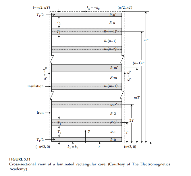
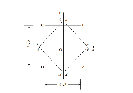
Figure 5.11 shows a rectangular core consisting of $n$-insulated laminations, each of width $W$ and overall thickness $T$. Let the insulation thickness on each side of a lamination be $T_1 / 2$ and its iron thickness be $T_2$. Further, let the corners of the rectangular core be located at $(-W / 2,0),(W / 2$, $0),(-W / 2, n T)$ and $(W / 2, n T)$. In this figure, insulation regions are indicated as Region- $0^{\prime}, 1^{\prime}, 2^{\prime}, 3^{\prime}, \ldots, m^{\prime}, \ldots, n^{\prime}$. The iron regions are indicated as Region- $1,2, \ldots, m, \ldots, n$.
The exciting coil is wound around the long rectangular core and carries an alternating current $i$, where $$ i=I e^{j \omega t} $$ It is simulated by a surface current density $K_o$ : $$ K_o=I \cdot N $$
where $N$ is the number of turns per unit length of the coil. The currentcarrying coil will produce time-varying magnetic field, $H_z$, in the core and eddy current density with components $J_x$ and $J_{y^{\prime}}$ in the conducting regions and displacement currents in the insulation regions of the core. The magnetic field outside the coil is neglected. For the long rectangular core with a uniformly distributed current sheet, the magnetic field is entirely axial and independent of $z$-coordinate, along the axial direction. It is assumed that the permeability $\mu$, for the iron regions, permittivity $\varepsilon$, for the insulation regions and conductivity $\left(\sigma, \sigma^{\prime}\right)$, for both types of regions, are constant. Thus, from Maxwell’s equations for harmonic fields, in charge-free regions $$ \frac{\partial^2 H_z}{\partial x^2}+\frac{\partial^2 H_z}{\partial y^2}=-\gamma^2 H_z $$ for iron regions, where $$ \gamma=\sqrt{(-j \omega \mu) \cdot\left(\sigma+j \omega \varepsilon_o\right)} $$ and $$ \frac{\partial^2 H_z}{\partial x^2}+\frac{\partial^2 H_z}{\partial y^2}=-\left(\gamma^{\prime}\right)^2 H_z $$ for insulation regions, where $$ \gamma^{\prime}=\sqrt{\left(-j \omega \mu_o\right) \cdot\left(\sigma^{\prime}+j \omega \varepsilon\right)} $$
物理代写|电磁学代写electromagnetism代考|Two-Dimensional Fields in Anisotropic Media
Consider an anisotropic homogeneous medium characterised by conductivity $[\sigma]$, permeability $[\mu]$ and permittivity $[\epsilon]$, such that $$ \begin{gathered} {[\sigma]=\left(\sigma_x, \sigma_y, \sigma_z\right)} \ {[\mu]=\left(\mu_x, \mu_y, \mu_z\right)} \ {[\epsilon]=\left(\epsilon_x, \epsilon_y, \epsilon_z\right)} \end{gathered} $$ while the components of complex conductivity are defined as $$ \begin{aligned} & \bar{\sigma}_x \stackrel{\text { def }}{=} \sigma_x+j \omega \epsilon_x \ & \bar{\sigma}_y \stackrel{\text { def }}{=} \sigma_y+j \omega \epsilon_y \ & \bar{\sigma}_z \stackrel{\text { def }}{=} \sigma_z+j \omega \epsilon_z \end{aligned} $$ Let there be a two-dimensional electromagnetic field that is independent of $x$-coordinate, varies periodically with $y$-coordinate as well as with time-t. This variation is given by the factor $e^{j(\omega t-(y)}$, where the time period is $2 \pi / \omega$ and the wave length is $2 \pi / \ell$, that is, two pole-pitches. To determine field variation with $z$-coordinate, we proceed with the Maxwell equation: $$ \nabla \times H=J+\frac{\partial D}{\partial t} $$ Thus, $$ \begin{aligned} & \frac{\partial H_z}{\partial y}-\frac{\partial H_y}{\partial z}=\bar{\sigma}_x E_x \ & \frac{\partial H_x}{\partial z}-\frac{\partial H_z}{\partial x}=\bar{\sigma}_y E_y \ & \frac{\partial H_y}{\partial x}-\frac{\partial H_x}{\partial y}=\bar{\sigma}_z E_z \end{aligned} $$
物理代写|电磁学代写electromagnetism代考|Eddy Currents in Laminated Rectangular Cores
物理代写|电磁学代写electromagnetism代考|Eddy Currents in Cores with Regular Polygonal Cross-Sections
物理代写|电磁学代写electromagnetism代考|Eddy Currents in Cores with Regular Polygonal Cross-Sections
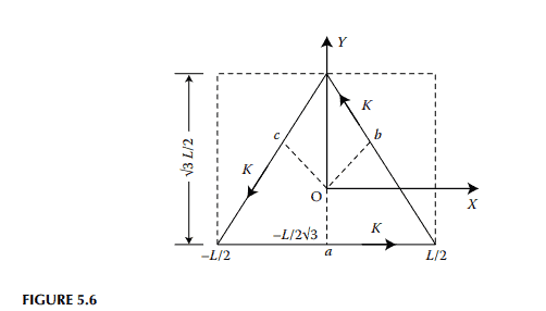
Distributions of magnetic fields in solid cores with rectangular and circular cross-sections due to alternating current excitation have been analytically determined. ${ }^{2,3}$ For cores with uncommon cross-sections, field distributions are usually evaluated using numerical methods., ${ }^{4,8}$ Analytical solutions are available $e^{5-7}$ for field distributions in cores with cross-sections in the shape of isosceles right-angled triangles. A quasi-analytical method for the determination of the approximate distribution of magnetic field intensity in cores with regular polygonal cross-sections is presented in this section as an alternative to the existing numerical methods. Although only three types of core sections, namely, cores with triangular, hexagonal and octagonal cross-sections, as shown in Figures 5.6 through 5.8 are considered, the method can be readily extended for other regular polygonal sections.
Consider a long conducting core carrying a surface current sheet with density $K$ simulating a uniformly distributed current-carrying winding wound around the core. The winding current is at power frequency. The magnetic field outside the core will be zero if the displacement currents are neglected. Inside the core, the magnetic field will be axial, that is in the $z$-direction such that just under the current sheet $$ \left.H_z\right|_{\text {core surface }}=K $$ where $|K|$ indicates the root mean square (rms) value of the surface current density on the conductor surface flowing in the anticlockwise direction, and $\mathrm{H}_z$ indicates the magnetic field in the axial direction, both in phasor form. The eddy current equation for the magnetic field is $$ \nabla^2 H_z=\eta^2 H_z $$ where $$ \eta^2=j \omega_0 \cdot \mu \sigma $$ $\omega_0=$ frequency of the sinusoidally time-varying field $\mu=$ permeability of the core $\sigma=$ conductivity of the core This is a two-dimensional problem as fields vary along $x$ – and $y$-directions only. Thus, $$ \frac{\partial H_z}{\partial x^2}+\frac{\partial H_z}{\partial y^2}=\eta^2 H_z $$ The solutions of this equation for solid cores with triangular, hexagonal and octagonal cross-sections are discussed in the following three subsections.
物理代写|电磁学代写electromagnetism代考|Cores with Triangular Cross-Sections
Consider a long solid-conducting core with a triangular cross-section shown in Figure 5.6. Let the length of each side of the triangle be $L$. A rectangle constructed using the base of this equilateral triangle is shown by dotted lines. Let the torch function be defined by the finite Fourier series: $$ \left.H_z^{\prime}\right|{y=L / \sqrt{3}}=\sum{m-\text { odd }}^{(2 M-1)} T_m \cdot \cos \left(\frac{m \pi}{L} \cdot x\right) $$ where $T_m$ indicates a set of Fourier coefficients.
On setting $$ \left.H_z^{\prime}\right|{x= \pm L / 2}=\left.H_z^{\prime}\right|{y=-L /(2 \sqrt{3})}=0 $$ The solution of eddy current equation for the rectangular region can be given as $$ H_z^{\prime}=\sum_{m-\alpha d d d}^{(2 M-1)} T_m \cdot \cos \left(\frac{m \pi}{L} \cdot x^{\prime}\right) \cdot \frac{\sinh \left[\alpha_m \cdot\left{y^{\prime}+L /(2 \sqrt{ } 3)\right}\right]}{\sinh \left(\alpha_m \cdot L \sqrt{3} / 2\right)} $$ where $$ \begin{gathered} \alpha_m=\sqrt{\left(\frac{m \pi}{L}\right)^2+\eta^2} \ x^{\prime}=x \ y^{\prime}=y \end{gathered} $$ Next, we construct two more similar rectangles, each containing one or the other of the two remaining sides of the equilateral triangle. Let the field distributions in these regions be $$ H_z^{\prime \prime}=\sum_{m-\text {-odd }}^{(2 M-1)} T_m \cdot \cos \left(\frac{m \pi}{L} \cdot x^{\prime \prime}\right) \cdot \frac{\sinh \left[\alpha_m \cdot\left{y^{\prime \prime}+L /(2 \sqrt{3})\right}\right]}{\sinh \left(\alpha_m \cdot L \cdot \sqrt{3} / 2\right)} $$


![数学代写|现代代数代写Modern Algebra代考|Mignotte’s factor bound and a modular gcd algorithm in Z[x]](https://www.statistics-lab.com/wp-content/uploads/2023/06/hqdefault-2.jpg)