如果你也在 怎样代写时间序列分析Time-Series Analysis 这个学科遇到相关的难题,请随时右上角联系我们的24/7代写客服。时间序列分析Time-Series Analysis是在数学中,是按时间顺序索引(或列出或绘制)的一系列数据点。最常见的是,一个时间序列是在连续的等距的时间点上的一个序列。因此,它是一个离散时间数据的序列。时间序列的例子有海洋潮汐的高度、太阳黑子的数量和道琼斯工业平均指数的每日收盘值。
时间序列分析Time-Series Analysis分析包括分析时间序列数据的方法,以提取有意义的统计数据和数据的其他特征。时间序列预测是使用一个模型来预测基于先前观察到的值的未来值。虽然经常采用回归分析的方式来测试一个或多个不同时间序列之间的关系,但这种类型的分析通常不被称为 “时间序列分析”,它特别指的是单一序列中不同时间点之间的关系。中断的时间序列分析是用来检测一个时间序列从之前到之后的演变变化,这种变化可能会影响基础变量。
statistics-lab™ 为您的留学生涯保驾护航 在代写时间序列分析Time-Series Analysis方面已经树立了自己的口碑, 保证靠谱, 高质且原创的统计Statistics代写服务。我们的专家在代写时间序列分析Time-Series Analysis代写方面经验极为丰富,各种代写时间序列分析Time-Series Analysis相关的作业也就用不着说。

统计代写|时间序列分析代写Time-Series Analysis代考|Factor analysis
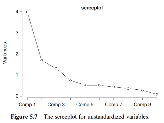
To build a factor model, we can either use the principle components method or maximum likelihood estimation method. However, for our data set, we have a vector series with a dimension $m=44$ and $n=30$. Its maximum likelihood equation cannot be properly solved. So, we can only use the principle component method. Thus, we will use PCA to estimate factors. In this analysis, we will follow Bai and Ng (2002), and select six factors, which is supported by the screeplot shown in Figure 5.5.
From the PCA analysis in Section 5.7.1, we will choose a factor model with six common factors,
$$
F_{1, t}=\operatorname{Comp} \cdot 1, F_{2, t}=\operatorname{Comp} \cdot 2, F_{3, t}=\operatorname{Comp} \cdot 3, F_{4, t}=\operatorname{Comp} \cdot 4, F_{5, t}=\operatorname{Comp} \cdot 5, F_{6, t}=\operatorname{Comp} \cdot 6
$$
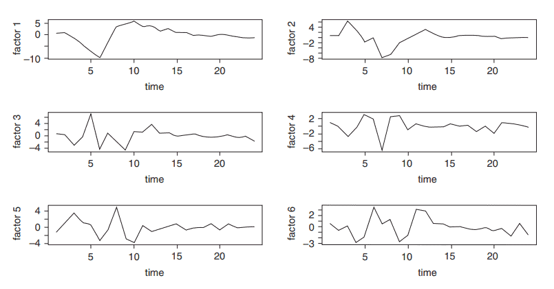
based on the standardized variables. The corresponding factor loadings, communalities, and specific variables are given in Table 5.8. The six estimated factor scores are plotted in Figure 5.9.
So, we have our factor model for the STD data set,
$$
\underset{44 \times 1}{\mathbf{Z}t}=\underset{(44 \times 6)}{\mathbf{L}} \underset{(6 \times 1)}{\mathbf{F}_t}+\underset{(44 \times 1)}{\boldsymbol{\varepsilon}_t}, $$ where the element and specification of $\mathbf{L}, \mathbf{F}_t$, and $\boldsymbol{\varepsilon}_t$ are given in Table 5.8. As described in Section 5.6, once values or scores of factors are estimated, we can combine the lagged values of $\mathbf{Z}_t$ or other observed variables in the model and build a forecast equation for the $h$-step ahead forecast for $\mathbf{Z}{t+h}$, that is
$$
\hat{\mathbf{Z}}_t(h)=\hat{\mathbf{\Pi}} \hat{\mathbf{F}}_t+\hat{\boldsymbol{\alpha}} \mathbf{V}_t
$$
where $\mathbf{V}_t$ are lagged values of $\mathbf{Z}_t$ and/or other observed variables, and $\hat{\boldsymbol{\Pi}}$ and $\hat{\boldsymbol{\alpha}}$ are the parameter estimates based on $\mathbf{V}_t$ given in Eq. (5.57).
In this example, we will simply choose $\mathbf{V}t$ to be the first lagged value of $\mathbf{Z}_t$. Specifically, our forecasting equations will be $$ \hat{Z}{i, t}(h)=\hat{\boldsymbol{\beta}}i^{\prime} \hat{\mathbf{F}}_t+\hat{\alpha}_i \hat{Z}{i, t}(h-1), i=1, \ldots, 44,
$$
where $\hat{\boldsymbol{\beta}}i^{\prime}$ is the $i$ th row of $\hat{\mathbf{\Pi}}$, and $\hat{\alpha}_i$ is the $i$ th element of $\hat{\boldsymbol{\alpha}}$. For $i=1$, we have $$ \hat{Z}{1, t}(h)=\hat{\boldsymbol{\beta}}1^{\prime} \hat{\mathbf{F}}_t+\hat{\alpha}_1 \hat{Z}{1, t}(h-1), t=1, \ldots, 24,
$$
and for $h=1$, it becomes
$$
\hat{Z}{1,24}(1)=\hat{\boldsymbol{\beta}}_1^{\prime} \hat{\mathbf{F}}_t+\hat{\alpha}_1 Z{1, t} .
$$
统计代写|时间序列分析代写Time-Series Analysis代考|VEC and DVEC models
For any square matrix $\mathbf{A}$, let vech(A) be the vector formed by stacking the elements of each column on or below the diagonal of $\mathbf{A}$. Thus,
$$
\operatorname{vech}\left[\begin{array}{lll}
\sigma_{1,1} & \sigma_{1,2} & \sigma_{1,3} \
\sigma_{2,1} & \sigma_{2,2} & \sigma_{2,3} \
\sigma_{3,1} & \sigma_{3,2} & \sigma_{3,3}
\end{array}\right]=\left[\begin{array}{l}
\sigma_{1,1} \
\sigma_{2,1} \
\sigma_{3,1} \
\sigma_{2,2} \
\sigma_{3,2} \
\sigma_{3,3}
\end{array}\right]
$$
Then the most natural extension of Eq. (6.2) to the ( $m \times 1)$ vector case in Eq. (6.5) is the following vector VEC model proposed by Bollerslev, Engle, and Wooldridge (1988)
$$
\operatorname{vech}\left(\boldsymbol{\Sigma}t\right)=\boldsymbol{\Theta}_0+\sum{j=1}^p \boldsymbol{\Phi}j \operatorname{vech}\left(\boldsymbol{\Sigma}{t-j}\right)+\sum_{j=1}^q \boldsymbol{\Theta}j \operatorname{vech}\left(\boldsymbol{\varepsilon}{t-j} \boldsymbol{\varepsilon}_{t-j}^{\prime}\right) .
$$
where each element of $\boldsymbol{\Sigma}_t$ is a function of lagged values of $\boldsymbol{\Sigma}_t$ and the squared and cross products of lagged variables or errors, $\boldsymbol{\Theta}_0$ is a $[m(m+1) / 2] \times 1$ column vector, and each of the coefficient matrices, $\boldsymbol{\Phi}j$ and $\boldsymbol{\Theta}_j$, is a $[m(m+1) / 2] \times[m(m+1) / 2]$ matrix. The model in Eq. (6.6) is known as $\operatorname{VEC}(p, q)$ model, and shown by Engle and Kroner (1995) it is stationary if and only if all eigenvalues of $\sum{j=1}^p \boldsymbol{\Phi}j+\sum{j=1}^q \boldsymbol{\Theta}j$ are within the unit circle. For example, the VEC(1,1) model is given by $$ \operatorname{vech}\left(\boldsymbol{\Sigma}_t\right)=\boldsymbol{\Theta}_0+\boldsymbol{\Phi}_1 \operatorname{vech}\left(\boldsymbol{\Sigma}{t-1}\right)+\boldsymbol{\Theta}1 \operatorname{vech}\left(\boldsymbol{\varepsilon}{t-1} \boldsymbol{\varepsilon}_{t-1}^{\prime}\right) .
$$
时间序列分析代考
统计代写|时间序列分析代写Time-Series Analysis代考|Factor analysis
建立因子模型可以采用主成分法,也可以采用极大似然估计法。然而,对于我们的数据集,我们有一个维度为$m=44$和$n=30$的向量序列。它的极大似然方程不能很好地求解。因此,我们只能采用主成分法。因此,我们将使用PCA来估计因子。在本分析中,我们将遵循Bai和Ng(2002),选择六个因素,并由图5.5所示的屏幕图支持。
从5.7.1节的主成分分析中,我们将选择一个具有六个共同因素的因子模型,
$$
F_{1, t}=\operatorname{Comp} \cdot 1, F_{2, t}=\operatorname{Comp} \cdot 2, F_{3, t}=\operatorname{Comp} \cdot 3, F_{4, t}=\operatorname{Comp} \cdot 4, F_{5, t}=\operatorname{Comp} \cdot 5, F_{6, t}=\operatorname{Comp} \cdot 6
$$
基于标准化变量。表5.8给出了相应的因子负载、社区和特定变量。6个估计因子得分如图5.9所示。
我们有STD数据集的因子模型,
$$
\underset{44 \times 1}{\mathbf{Z}t}=\underset{(44 \times 6)}{\mathbf{L}} \underset{(6 \times 1)}{\mathbf{F}_t}+\underset{(44 \times 1)}{\boldsymbol{\varepsilon}_t}, $$其中$\mathbf{L}, \mathbf{F}_t$和$\boldsymbol{\varepsilon}_t$的元素和规格如表5.8所示。如第5.6节所述,一旦估算出因子的值或分数,我们可以结合模型中$\mathbf{Z}_t$或其他观测变量的滞后值,构建预测方程,对$\mathbf{Z}{t+h}$进行$h$步前预测,即
$$
\hat{\mathbf{Z}}_t(h)=\hat{\mathbf{\Pi}} \hat{\mathbf{F}}_t+\hat{\boldsymbol{\alpha}} \mathbf{V}_t
$$
其中$\mathbf{V}_t$为$\mathbf{Z}_t$和/或其他观测变量的滞后值,$\hat{\boldsymbol{\Pi}}$和$\hat{\boldsymbol{\alpha}}$为式(5.57)中基于$\mathbf{V}_t$的参数估计。
在本例中,我们将简单地选择$\mathbf{V}t$作为$\mathbf{Z}_t$的第一个滞后值。具体来说,我们的预测方程是$$ \hat{Z}{i, t}(h)=\hat{\boldsymbol{\beta}}i^{\prime} \hat{\mathbf{F}}_t+\hat{\alpha}_i \hat{Z}{i, t}(h-1), i=1, \ldots, 44,
$$
其中$\hat{\boldsymbol{\beta}}i^{\prime}$是$\hat{\mathbf{\Pi}}$的第$i$行,$\hat{\alpha}_i$是$\hat{\boldsymbol{\alpha}}$的第$i$个元素。对于$i=1$,我们有$$ \hat{Z}{1, t}(h)=\hat{\boldsymbol{\beta}}1^{\prime} \hat{\mathbf{F}}_t+\hat{\alpha}_1 \hat{Z}{1, t}(h-1), t=1, \ldots, 24,
$$
对于$h=1$,它变成
$$
\hat{Z}{1,24}(1)=\hat{\boldsymbol{\beta}}_1^{\prime} \hat{\mathbf{F}}_t+\hat{\alpha}_1 Z{1, t} .
$$
统计代写|时间序列分析代写Time-Series Analysis代考|VEC and DVEC models
对于任意方阵$\mathbf{A}$,设vech(A)是通过将每列的元素叠加在$\mathbf{A}$对角线上或下而形成的向量。因此,
$$
\operatorname{vech}\left[\begin{array}{lll}
\sigma_{1,1} & \sigma_{1,2} & \sigma_{1,3} \
\sigma_{2,1} & \sigma_{2,2} & \sigma_{2,3} \
\sigma_{3,1} & \sigma_{3,2} & \sigma_{3,3}
\end{array}\right]=\left[\begin{array}{l}
\sigma_{1,1} \
\sigma_{2,1} \
\sigma_{3,1} \
\sigma_{2,2} \
\sigma_{3,2} \
\sigma_{3,3}
\end{array}\right]
$$
那么,将Eq.(6.2)最自然地推广到Eq.(6.5)中的($m \times 1)$)向量情况就是Bollerslev, Engle和Wooldridge(1988)提出的向量VEC模型。
$$
\operatorname{vech}\left(\boldsymbol{\Sigma}t\right)=\boldsymbol{\Theta}0+\sum{j=1}^p \boldsymbol{\Phi}j \operatorname{vech}\left(\boldsymbol{\Sigma}{t-j}\right)+\sum{j=1}^q \boldsymbol{\Theta}j \operatorname{vech}\left(\boldsymbol{\varepsilon}{t-j} \boldsymbol{\varepsilon}{t-j}^{\prime}\right) . $$ 其中$\boldsymbol{\Sigma}_t$的每个元素是$\boldsymbol{\Sigma}_t$的滞后值以及滞后变量或误差的平方和叉乘的函数,$\boldsymbol{\Theta}_0$是一个$[m(m+1) / 2] \times 1$列向量,每个系数矩阵$\boldsymbol{\Phi}j$和$\boldsymbol{\Theta}_j$是一个$[m(m+1) / 2] \times[m(m+1) / 2]$矩阵。式(6.6)中的模型称为$\operatorname{VEC}(p, q)$模型,Engle和Kroner(1995)表明,当且仅当$\sum{j=1}^p \boldsymbol{\Phi}j+\sum{j=1}^q \boldsymbol{\Theta}j$的所有特征值都在单位圆内时,该模型是平稳的。例如,VEC(1,1)模型由 $$ \operatorname{vech}\left(\boldsymbol{\Sigma}_t\right)=\boldsymbol{\Theta}_0+\boldsymbol{\Phi}_1 \operatorname{vech}\left(\boldsymbol{\Sigma}{t-1}\right)+\boldsymbol{\Theta}1 \operatorname{vech}\left(\boldsymbol{\varepsilon}{t-1} \boldsymbol{\varepsilon}{t-1}^{\prime}\right) .
$$

统计代写请认准statistics-lab™. statistics-lab™为您的留学生涯保驾护航。
金融工程代写
金融工程是使用数学技术来解决金融问题。金融工程使用计算机科学、统计学、经济学和应用数学领域的工具和知识来解决当前的金融问题,以及设计新的和创新的金融产品。
非参数统计代写
非参数统计指的是一种统计方法,其中不假设数据来自于由少数参数决定的规定模型;这种模型的例子包括正态分布模型和线性回归模型。
广义线性模型代考
广义线性模型(GLM)归属统计学领域,是一种应用灵活的线性回归模型。该模型允许因变量的偏差分布有除了正态分布之外的其它分布。
术语 广义线性模型(GLM)通常是指给定连续和/或分类预测因素的连续响应变量的常规线性回归模型。它包括多元线性回归,以及方差分析和方差分析(仅含固定效应)。
有限元方法代写
有限元方法(FEM)是一种流行的方法,用于数值解决工程和数学建模中出现的微分方程。典型的问题领域包括结构分析、传热、流体流动、质量运输和电磁势等传统领域。
有限元是一种通用的数值方法,用于解决两个或三个空间变量的偏微分方程(即一些边界值问题)。为了解决一个问题,有限元将一个大系统细分为更小、更简单的部分,称为有限元。这是通过在空间维度上的特定空间离散化来实现的,它是通过构建对象的网格来实现的:用于求解的数值域,它有有限数量的点。边界值问题的有限元方法表述最终导致一个代数方程组。该方法在域上对未知函数进行逼近。[1] 然后将模拟这些有限元的简单方程组合成一个更大的方程系统,以模拟整个问题。然后,有限元通过变化微积分使相关的误差函数最小化来逼近一个解决方案。
tatistics-lab作为专业的留学生服务机构,多年来已为美国、英国、加拿大、澳洲等留学热门地的学生提供专业的学术服务,包括但不限于Essay代写,Assignment代写,Dissertation代写,Report代写,小组作业代写,Proposal代写,Paper代写,Presentation代写,计算机作业代写,论文修改和润色,网课代做,exam代考等等。写作范围涵盖高中,本科,研究生等海外留学全阶段,辐射金融,经济学,会计学,审计学,管理学等全球99%专业科目。写作团队既有专业英语母语作者,也有海外名校硕博留学生,每位写作老师都拥有过硬的语言能力,专业的学科背景和学术写作经验。我们承诺100%原创,100%专业,100%准时,100%满意。
随机分析代写
随机微积分是数学的一个分支,对随机过程进行操作。它允许为随机过程的积分定义一个关于随机过程的一致的积分理论。这个领域是由日本数学家伊藤清在第二次世界大战期间创建并开始的。
时间序列分析代写
随机过程,是依赖于参数的一组随机变量的全体,参数通常是时间。 随机变量是随机现象的数量表现,其时间序列是一组按照时间发生先后顺序进行排列的数据点序列。通常一组时间序列的时间间隔为一恒定值(如1秒,5分钟,12小时,7天,1年),因此时间序列可以作为离散时间数据进行分析处理。研究时间序列数据的意义在于现实中,往往需要研究某个事物其随时间发展变化的规律。这就需要通过研究该事物过去发展的历史记录,以得到其自身发展的规律。
回归分析代写
多元回归分析渐进(Multiple Regression Analysis Asymptotics)属于计量经济学领域,主要是一种数学上的统计分析方法,可以分析复杂情况下各影响因素的数学关系,在自然科学、社会和经济学等多个领域内应用广泛。
MATLAB代写
MATLAB 是一种用于技术计算的高性能语言。它将计算、可视化和编程集成在一个易于使用的环境中,其中问题和解决方案以熟悉的数学符号表示。典型用途包括:数学和计算算法开发建模、仿真和原型制作数据分析、探索和可视化科学和工程图形应用程序开发,包括图形用户界面构建MATLAB 是一个交互式系统,其基本数据元素是一个不需要维度的数组。这使您可以解决许多技术计算问题,尤其是那些具有矩阵和向量公式的问题,而只需用 C 或 Fortran 等标量非交互式语言编写程序所需的时间的一小部分。MATLAB 名称代表矩阵实验室。MATLAB 最初的编写目的是提供对由 LINPACK 和 EISPACK 项目开发的矩阵软件的轻松访问,这两个项目共同代表了矩阵计算软件的最新技术。MATLAB 经过多年的发展,得到了许多用户的投入。在大学环境中,它是数学、工程和科学入门和高级课程的标准教学工具。在工业领域,MATLAB 是高效研究、开发和分析的首选工具。MATLAB 具有一系列称为工具箱的特定于应用程序的解决方案。对于大多数 MATLAB 用户来说非常重要,工具箱允许您学习和应用专业技术。工具箱是 MATLAB 函数(M 文件)的综合集合,可扩展 MATLAB 环境以解决特定类别的问题。可用工具箱的领域包括信号处理、控制系统、神经网络、模糊逻辑、小波、仿真等。