
如果你也在 怎样代写时间序列分析Time-Series Analysis 这个学科遇到相关的难题,请随时右上角联系我们的24/7代写客服。时间序列分析Time-Series Analysis是在数学中,是按时间顺序索引(或列出或绘制)的一系列数据点。最常见的是,一个时间序列是在连续的等距的时间点上的一个序列。因此,它是一个离散时间数据的序列。时间序列的例子有海洋潮汐的高度、太阳黑子的数量和道琼斯工业平均指数的每日收盘值。
时间序列分析Time-Series Analysis分析包括分析时间序列数据的方法,以提取有意义的统计数据和数据的其他特征。时间序列预测是使用一个模型来预测基于先前观察到的值的未来值。虽然经常采用回归分析的方式来测试一个或多个不同时间序列之间的关系,但这种类型的分析通常不被称为 “时间序列分析”,它特别指的是单一序列中不同时间点之间的关系。中断的时间序列分析是用来检测一个时间序列从之前到之后的演变变化,这种变化可能会影响基础变量。
statistics-lab™ 为您的留学生涯保驾护航 在代写时间序列分析Time-Series Analysis方面已经树立了自己的口碑, 保证靠谱, 高质且原创的统计Statistics代写服务。我们的专家在代写时间序列分析Time-Series Analysis代写方面经验极为丰富,各种代写时间序列分析Time-Series Analysis相关的作业也就用不着说。
统计代写|时间序列分析代写Time-Series Analysis代考|Vehicular theft data
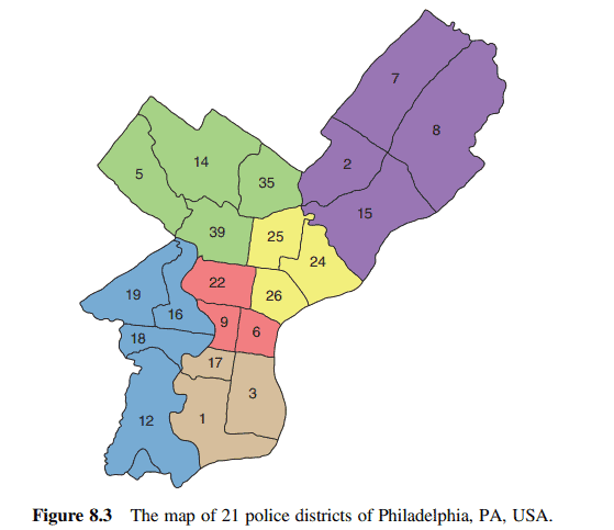
Example 8.5 From January 2006 through December 2014, over 750,000 crimes were reported among the 21 police districts in Philadelphia, Pennsylvania, shown on the map in Figure 8.3. The most common crimes reported were thefts and burglaries. The total crime followed a seasonal pattern with more crimes in the summer than in the winter.
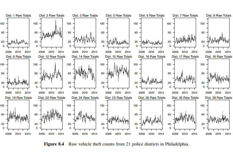
For this analysis, we consider the monthly total of vehicle thefts recorded at the 21 police districts in Philadelphia from January 2006 to December 2014. The data set consists of $m=21$ dimensions corresponding to the 21 police districts and is listed as WW8a in the Data Appendix. The monthly total of vehicle thefts from January 2006 to April 2014 was used for model fitting with a total of $n=100$ observations. The monthly total of the thefts from May 2014 to December 2014 was held out for the forecast comparison. Figure 8.4 displays these raw counts for the in-sample time points.
Visually, each time series shows a constant mean but varies among districts. For the variance, we compare several values for the Box-Cox transformation, and $\lambda=0.5$ is chosen for most locations to stabilize the variance. Thus, the square root of each series was performed. Neither regular nor seasonal differencing was required for any of the 21 series. After being square-root-transformed and mean centered, the resulting 21 series for $t=1,2, \ldots, 100$, is given in Figure 8.5.
Bordering districts are defined as first neighbors, and the weighting matrix for $\mathbf{W}^{(1)}$ is given in Table 8.2. Models involving additional spatial lags were considered but the parameter estimates were not significant different from 0 , and hence the weighting matrices $\mathbf{W}^{(\ell)}$ for $\ell>1$ are not given.
The patterns in Figure 8.6 show that the sample ST-ACFs exponentially decay at both regular time lags, seasonal time lags of multiple of 12 , and that ST-PACFs are significant only at time lags 2,12 , and 24 , and spatial lag at 1 . For a monthly series of seasonal period of 12 , we tentatively choose a $\operatorname{STAR}\left(2_{1,1}\right) \times\left(2_{1,1}\right)_{12}$ as its possible underlying model. The estimation result is given as follows:
Since the estimate of $\phi_{2,1}$ is only 1.46 standard errors away from 0 , we re-fit a STAR $\left(2_{1,0}\right) \times\left(2_{1,1}\right){12}$ model with the following result, $$ \begin{aligned} & \left(\mathbf{I}{21}-\underset{(.031)}{0.128} \mathbf{W}^{(0)} B^{12}-\underset{(.063)}{0.145 \mathbf{W}^{(1)}} B^{12}-\underset{(.033)}{0.058} \mathbf{W}^{(0)} B^{24}-\underset{(.067)}{0.149 \mathbf{W}^{(1)} B^{24}}\right) \
& \left(\mathbf{I}_{21}-\underset{(.029)}{0.336} \mathbf{W}^{(0)} B-\underset{(056)}{0.171 \mathbf{W}^{(1)}} B-\underset{(.034)}{0.121 \mathbf{W}^{(0)}} B^2\right) \mathbf{Z}_t=\mathbf{a}_t . \
&
\end{aligned}
$$
统计代写|时间序列分析代写Time-Series Analysis代考|The annual U.S. labor force count
Example 8.6 The United States Department of Labor provides dozens of variables through the Bureau of Labor Statistics (BLS), many of which could be fitted with various STARMA models. We select non-seasonally adjusted labor force count for the 48 contiguous states and Washington D.C., for a total of $m=49$ locations. The data are annual from 1976 through 2014 . This constitutes our raw data, which is listed as WW8b in the Data Appendix.
To arrive at the variable $\mathbf{Z}_t$, we already tested and determined that most of the individual time series variables were variance stationary, but appear to have a single unit root. Thus, we took the difference of the counts, and then mean centered the variable for each location. This gives us our zero-mean variable $\mathbf{Z}_t$, with dimension $m=49$ and time points $n=39$. As a side note, one reason for a STARMA-type model to be beneficial for this data is that a VAR(1) model would require $49 \times 49=2401$ parameters, which are more than the number of observations in the data set, and makes the regular VAR fitting impossible. However, the same first order STAR $\left(1_1\right)$ model involves only two parameters.
First, we construct the weighting matrix $\mathbf{W}^{(1)}$ according to the number of bordering states (first neighbors) each state has. Though too large to include for each state in this example, the number of border states ranges from 1 (Maine) to 8 (Missouri and Tennessee). And although not shown, we also construct $\mathbf{W}^{(2)}$ and $\mathbf{W}^{(3)}$ regarding second and third neighbors. Second neighbors are states that do not border each other but have at least one first neighbor in common. These terms are not needed for the chosen STAR $\left(1_1\right)$ model in this example but are included to see if the spatial order is indeed only 1 . Actually, these matrices allow us to construct the sample ST-ACF and ST-PACF, as shown in Tables 8.3 and 8.4.
时间序列分析代考
统计代写|时间序列分析代写Time-Series Analysis代考|Vehicular theft data
从2006年1月到2014年12月,宾夕法尼亚州费城的21个警区报告了超过75万起犯罪,如图8.3所示。最常见的犯罪是盗窃和入室行窃。犯罪总量有季节性规律,夏季犯罪比冬季多。
为了进行分析,我们考虑了2006年1月至2014年12月在费城21个警察区记录的每月车辆盗窃案总数。该数据集由与21个警区相对应的$m=21$维度组成,在数据附录中列为WW8a。从2006年1月到2014年4月的每月车辆盗窃总数用于模型拟合,总共有$n=100$观测值。2014年5月至2014年12月的月度盗窃案总数用于预测比较。图8.4显示了样本内时间点的原始计数。
从视觉上看,每个时间序列显示一个恒定的平均值,但在地区之间有所不同。对于方差,我们比较了Box-Cox变换的几个值,对于大多数位置选择$\lambda=0.5$来稳定方差。因此,每个级数的平方根被执行。21个系列中的任何一个都不需要常规或季节差异。经过平方根变换并以均值为中心后,得到$t=1,2, \ldots, 100$的21级数如图8.5所示。
将邻域定义为第一邻域,$\mathbf{W}^{(1)}$的权重矩阵如表8.2所示。考虑了涉及额外空间滞后的模型,但参数估计与0没有显著差异,因此没有给出$\ell>1$的权重矩阵$\mathbf{W}^{(\ell)}$。
从图8.6的模式可以看出,样品ST-PACFs在常规时间滞后和12倍的季节性时间滞后下都呈指数衰减,ST-PACFs仅在时间滞后2、12和24时显著,在空间滞后1时显著。对于12个季节周期的月度序列,我们暂时选择$\operatorname{STAR}\left(2_{1,1}\right) \times\left(2_{1,1}\right)_{12}$作为其可能的基础模型。估计结果如下:
由于$\phi_{2,1}$的估计值离0只有1.46个标准误差,我们用以下结果重新拟合STAR $\left(2_{1,0}\right) \times\left(2_{1,1}\right){12}$模型: $$ \begin{aligned} & \left(\mathbf{I}{21}-\underset{(.031)}{0.128} \mathbf{W}^{(0)} B^{12}-\underset{(.063)}{0.145 \mathbf{W}^{(1)}} B^{12}-\underset{(.033)}{0.058} \mathbf{W}^{(0)} B^{24}-\underset{(.067)}{0.149 \mathbf{W}^{(1)} B^{24}}\right) \
& \left(\mathbf{I}_{21}-\underset{(.029)}{0.336} \mathbf{W}^{(0)} B-\underset{(056)}{0.171 \mathbf{W}^{(1)}} B-\underset{(.034)}{0.121 \mathbf{W}^{(0)}} B^2\right) \mathbf{Z}_t=\mathbf{a}_t . \
&
\end{aligned}
$$
统计代写|时间序列分析代写Time-Series Analysis代考|The annual U.S. labor force count
例8.6美国劳工部通过劳工统计局(BLS)提供了几十个变量,其中许多变量可以用各种STARMA模型进行拟合。我们选择48个连续州和华盛顿特区的非季节性调整劳动力数量,总共$m=49$地点。这些数据是从1976年到2014年的年度数据。这构成了我们的原始数据,在数据附录中被列为WW8b。
为了得到变量$\mathbf{Z}_t$,我们已经测试并确定了大多数单独的时间序列变量是方差平稳的,但似乎有一个单一的单位根。因此,我们取计数的差值,然后对每个位置的变量平均居中。这给了我们零均值变量$\mathbf{Z}_t$,维度$m=49$和时间点$n=39$。作为附带说明,starma类型模型对该数据有益的一个原因是VAR(1)模型需要$49 \times 49=2401$参数,这些参数超过数据集中的观测值数量,并且使常规VAR拟合不可能。然而,相同的一阶STAR $\left(1_1\right)$模型只涉及两个参数。
首先,我们根据每个状态的边界状态(第一邻居)的数量构造加权矩阵$\mathbf{W}^{(1)}$。虽然这个例子中没有包括每个州,但边境州的数量从1个(缅因州)到8个(密苏里州和田纳西州)不等。虽然没有显示出来,我们也构造了$\mathbf{W}^{(2)}$和$\mathbf{W}^{(3)}$关于第二个和第三个邻居。第二邻国是指不相邻但至少有一个共同的第一邻国的国家。在本例中,所选的STAR $\left(1_1\right)$模型不需要这些术语,但包含这些术语是为了查看空间顺序是否确实只有1。实际上,这些矩阵允许我们构建样本ST-ACF和ST-PACF,如表8.3和8.4所示。

统计代写请认准statistics-lab™. statistics-lab™为您的留学生涯保驾护航。
金融工程代写
金融工程是使用数学技术来解决金融问题。金融工程使用计算机科学、统计学、经济学和应用数学领域的工具和知识来解决当前的金融问题,以及设计新的和创新的金融产品。
非参数统计代写
非参数统计指的是一种统计方法,其中不假设数据来自于由少数参数决定的规定模型;这种模型的例子包括正态分布模型和线性回归模型。
广义线性模型代考
广义线性模型(GLM)归属统计学领域,是一种应用灵活的线性回归模型。该模型允许因变量的偏差分布有除了正态分布之外的其它分布。
术语 广义线性模型(GLM)通常是指给定连续和/或分类预测因素的连续响应变量的常规线性回归模型。它包括多元线性回归,以及方差分析和方差分析(仅含固定效应)。
有限元方法代写
有限元方法(FEM)是一种流行的方法,用于数值解决工程和数学建模中出现的微分方程。典型的问题领域包括结构分析、传热、流体流动、质量运输和电磁势等传统领域。
有限元是一种通用的数值方法,用于解决两个或三个空间变量的偏微分方程(即一些边界值问题)。为了解决一个问题,有限元将一个大系统细分为更小、更简单的部分,称为有限元。这是通过在空间维度上的特定空间离散化来实现的,它是通过构建对象的网格来实现的:用于求解的数值域,它有有限数量的点。边界值问题的有限元方法表述最终导致一个代数方程组。该方法在域上对未知函数进行逼近。[1] 然后将模拟这些有限元的简单方程组合成一个更大的方程系统,以模拟整个问题。然后,有限元通过变化微积分使相关的误差函数最小化来逼近一个解决方案。
tatistics-lab作为专业的留学生服务机构,多年来已为美国、英国、加拿大、澳洲等留学热门地的学生提供专业的学术服务,包括但不限于Essay代写,Assignment代写,Dissertation代写,Report代写,小组作业代写,Proposal代写,Paper代写,Presentation代写,计算机作业代写,论文修改和润色,网课代做,exam代考等等。写作范围涵盖高中,本科,研究生等海外留学全阶段,辐射金融,经济学,会计学,审计学,管理学等全球99%专业科目。写作团队既有专业英语母语作者,也有海外名校硕博留学生,每位写作老师都拥有过硬的语言能力,专业的学科背景和学术写作经验。我们承诺100%原创,100%专业,100%准时,100%满意。
随机分析代写
随机微积分是数学的一个分支,对随机过程进行操作。它允许为随机过程的积分定义一个关于随机过程的一致的积分理论。这个领域是由日本数学家伊藤清在第二次世界大战期间创建并开始的。
时间序列分析代写
随机过程,是依赖于参数的一组随机变量的全体,参数通常是时间。 随机变量是随机现象的数量表现,其时间序列是一组按照时间发生先后顺序进行排列的数据点序列。通常一组时间序列的时间间隔为一恒定值(如1秒,5分钟,12小时,7天,1年),因此时间序列可以作为离散时间数据进行分析处理。研究时间序列数据的意义在于现实中,往往需要研究某个事物其随时间发展变化的规律。这就需要通过研究该事物过去发展的历史记录,以得到其自身发展的规律。
回归分析代写
多元回归分析渐进(Multiple Regression Analysis Asymptotics)属于计量经济学领域,主要是一种数学上的统计分析方法,可以分析复杂情况下各影响因素的数学关系,在自然科学、社会和经济学等多个领域内应用广泛。
MATLAB代写
MATLAB 是一种用于技术计算的高性能语言。它将计算、可视化和编程集成在一个易于使用的环境中,其中问题和解决方案以熟悉的数学符号表示。典型用途包括:数学和计算算法开发建模、仿真和原型制作数据分析、探索和可视化科学和工程图形应用程序开发,包括图形用户界面构建MATLAB 是一个交互式系统,其基本数据元素是一个不需要维度的数组。这使您可以解决许多技术计算问题,尤其是那些具有矩阵和向量公式的问题,而只需用 C 或 Fortran 等标量非交互式语言编写程序所需的时间的一小部分。MATLAB 名称代表矩阵实验室。MATLAB 最初的编写目的是提供对由 LINPACK 和 EISPACK 项目开发的矩阵软件的轻松访问,这两个项目共同代表了矩阵计算软件的最新技术。MATLAB 经过多年的发展,得到了许多用户的投入。在大学环境中,它是数学、工程和科学入门和高级课程的标准教学工具。在工业领域,MATLAB 是高效研究、开发和分析的首选工具。MATLAB 具有一系列称为工具箱的特定于应用程序的解决方案。对于大多数 MATLAB 用户来说非常重要,工具箱允许您学习和应用专业技术。工具箱是 MATLAB 函数(M 文件)的综合集合,可扩展 MATLAB 环境以解决特定类别的问题。可用工具箱的领域包括信号处理、控制系统、神经网络、模糊逻辑、小波、仿真等。