标签： KYA322

物理代写|固体物理代写Solid-state physics代考|PH581

Posted on 2023年8月8日2023年8月8日 by statistics-lab

如果你也在怎样代写固体物理Solid Physics PHYS881这个学科遇到相关的难题，请随时右上角联系我们的24/7代写客服。固体物理Solid Physics是通过量子力学、晶体学、电磁学和冶金学等方法研究刚性物质或固体。它是凝聚态物理学的最大分支。固体物理学研究固体材料的大尺度特性是如何产生于其原子尺度特性的。因此，固态物理学构成了材料科学的理论基础。它也有直接的应用，例如在晶体管和半导体的技术中。

固体物理Solid Physics是由密密麻麻的原子形成的，这些原子之间有强烈的相互作用。这些相互作用产生了固体的机械（如硬度和弹性）、热、电、磁和光学特性。根据所涉及的材料及其形成的条件，原子可能以有规律的几何模式排列（晶体固体，包括金属和普通水冰）或不规则地排列（非晶体固体，如普通窗玻璃）。

statistics-lab™ 为您的留学生涯保驾护航在代写固体物理Solid-state physics方面已经树立了自己的口碑, 保证靠谱, 高质且原创的统计Statistics代写服务。我们的专家在代写固体物理Solid-state physics代写方面经验极为丰富，各种代写固体物理Solid-state physics相关的作业也就用不着说。

物理代写|固体物理代写Solid-state physics代考|Semiconductor Doping

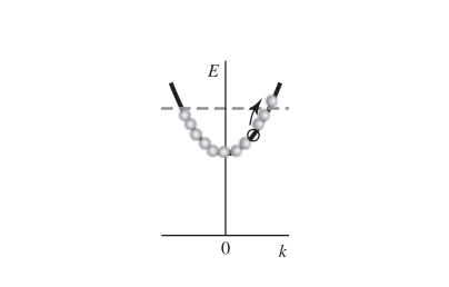
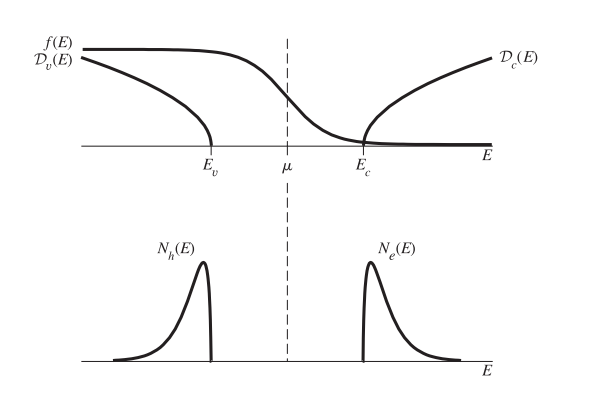
In a typical semiconductor with a band gap of $1-2 \mathrm{eV}$, very few electrons will be thermally excited enough to jump from the valence band to the conduction band. It is possible to get free carriers in another way, however, by selective doping of the material.

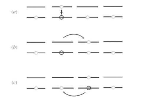
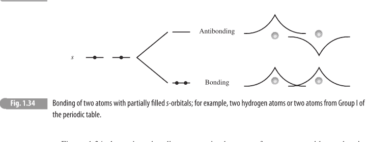
As discussed in Section 1.11.2, typical semiconductors are made from II-VI, III-V or Group IV elements, which have eight electrons per unit cell filling eight molecular bonding states. Suppose that in a III-V semiconductor, we replace a single atom with one from Group VI. This atom will have an extra electron and an extra positive charge on its nucleus. It makes sense that the extra electron will tend to stay near the nucleus with the extra charge, but if the energy of the extra electron is high enough, it may leave the dopant atom and migrate through the crystal as a free quasiparticle.

As in the case of excitons, if the dielectric constant of the material is high, then the bound states of carriers at an impurity can be viewed as hydrogen-like states of a carrier orbiting a charged particle. If a dopant nucleus has one extra positive charge relative to the atom it replaces in the lattice, then a negative electron will see a single positive charge sitting in the background “vacuum” of the normal band structure of the material. It can then orbit this positive charge in a hydrogenic state with a binding energy given by (2.3.5). The reduced mass in this case will just be the effective mass of the electron, because the impurity cannot move, and therefore it effectively has infinite mass.

In the same way, a dopant nucleus with one less charge than the one it replaces in the lattice will look like a single negative charge to the quasiparticles. Therefore, a hole can orbit this atom in a hydrogenic bound state. Again, the negative impurity has effectively infinite mass because it cannot move, and so the binding energy of the hole will simply be proportional to the mass of the hole, according to (2.3.5) and (2.3.6).

At high temperature, that is, when $k_B T$ is much greater than the binding energy of a carrier orbiting an impurity, the carriers will no longer be bound to the impurities and will move freely through the crystal. Therefore, an atom with more positive charge on its nucleus than the one it replaces contributes an electron to the conduction band. This type of impurity is therefore called a charge donor, and a semiconductor doped with this type of atom is called $\boldsymbol{n}$-type (for “negative”). In the same way, an atom with a nucleus with more negative charge than the one it replaces contributes a hole to the valence band, which is the same as accepting an electron from the valence band. This type of impurity is therefore called an electron acceptor, and a semiconductor doped with this type of atom is called “p-type” (for “positive”).

物理代写|固体物理代写Solid-state physics代考|EquilibriumPopulations in Doped Semiconductors

At $T=0$, each additional electron and hole will be in its ground state, orbiting the impurity atom from which it came. At higher temperature, however, these quasiparticles can leave their bound states and move freely through the material. The probability of this happening depends on the binding energy of the carrier on the impurity. As we did in Section 2.5.1, we can write a mass action equation for the equilibrium concentration of the quasiparticles. For example, for electrons from donor atoms, at low temperature we write
$$
N_e N_h=N_Q^{(e)} N_D e^{-\left(E_c-E_D\right) / k_B T},
$$
where $N_D$ is the number of donor states available to the holes. At high temperature, however, this equation will break down, because the assumption that $k_B T \ll\left(E_C-E_D\right)$ made in the derivation of (2.5.8) will no longer be true. As discussed at the end of Section 2.5.1, if the number of donor states is much less than the number of states in the conduction band, as is typically the case in doped semiconductors, the chemical potential will be pushed down toward the donor state energy. In this case, we must use the Fermi-Dirac occupation number for the holes in the donor states,
$$
N_h=N_D \frac{1}{e^{\left(\mu-E_D\right) / k_B T}+1} .
$$
This can be rewritten as
$$
\begin{aligned}
N_h & =N_D\left(1-\frac{1}{e^{\left(\mu-E_D\right) / k_B T}+1}\right) e^{-\left(\mu-E_D\right) / k_B T} \
& =N_D\left(1-f_h\left(E_D\right)\right) e^{-\left(\mu-E_D\right) / k_B T} \
& =\left(N_D-N_h\right) e^{-\left(\mu-E_D\right) / k_B T} .
\end{aligned}
$$

固体物理代写

物理代写|固体物理代写Solid-state physics代考|Semiconductor Doping

在带隙为$1-2 \mathrm{eV}$的典型半导体中，很少有电子会被热激发到足以从价带跳到导带。然而，通过选择性掺杂材料，也有可能以另一种方式获得自由载流子。

如第1.11.2节所述，典型的半导体由II-VI、III-V或IV族元素制成，每个单元电池有8个电子，填充8个分子键态。假设在III-V族半导体中，我们用一个来自VI族的原子代替一个原子。这个原子的原子核上会多出一个电子和一个正电荷。多余的电子会带着多余的电荷留在原子核附近，这是有道理的，但如果多余电子的能量足够高，它可能会离开掺杂原子，以自由的准粒子的形式在晶体中迁移。

在激子的情况下，如果材料的介电常数很高，那么杂质载流子的束缚态可以看作是载流子绕带电粒子运行的类氢态。如果一个掺杂核相对于它在晶格中取代的原子有一个额外的正电荷，那么一个负电子就会在材料正常带结构的背景“真空”中看到一个单一的正电荷。然后它就可以在氢原子状态下围绕这个正电荷运行，其结合能为(2.3.5)。在这种情况下，减少的质量就是电子的有效质量，因为杂质不能移动，因此它的有效质量是无限大的。

以同样的方式，一个比它在晶格中取代的原子核少带一个电荷的掺杂核对准粒子来说就像一个负电荷。因此，一个空穴可以在氢原子束缚状态下围绕这个原子运行。同样，负杂质实际上具有无限大的质量，因为它不能移动，因此根据式(2.3.5)和式(2.3.6)，空穴的结合能将简单地与空穴的质量成正比。

在高温下，即当$k_B T$远大于绕杂质轨道运行的载流子的结合能时，载流子将不再与杂质结合，并在晶体中自由移动。因此，原子核上带更多正电荷的原子比它所取代的原子向传导带贡献一个电子。因此，这种类型的杂质被称为电荷供体，掺杂这种类型原子的半导体被称为$\boldsymbol{n}$型(表示“负极”)。以同样的方式，一个原子核比它所取代的原子核带更多的负电荷的原子为价带贡献了一个空穴，这与从价带接受一个电子是一样的。因此，这种类型的杂质被称为电子受体，而掺杂这种原子的半导体被称为“p型”(即“正极”)。

物理代写|固体物理代写Solid-state physics代考|EquilibriumPopulations in Doped Semiconductors

在$T=0$，每一个额外的电子和空穴都将处于基态，围绕它原来的杂质原子运行。然而，在更高的温度下，这些准粒子可以离开它们的束缚状态，在材料中自由移动。这种情况发生的概率取决于载流子对杂质的结合能。正如我们在2.5.1节中所做的那样，我们可以写出准粒子平衡浓度的质量作用方程。例如，对于来自供体原子的电子，在低温下我们写
$$
N_e N_h=N_Q^{(e)} N_D e^{-\left(E_c-E_D\right) / k_B T},
$$
其中$N_D$是可供洞口使用的捐助国数目。然而，在高温下，这个方程将失效，因为在(2.5.8)的推导中所做的$k_B T \ll\left(E_C-E_D\right)$假设将不再成立。如第2.5.1节末尾所讨论的，如果施主态的数量远远少于导带中的状态数，如掺杂半导体中的典型情况，则化学势将被向下推至施主态能量。在这种情况下，我们必须使用费米-狄拉克占用数来表示供体态中的空穴，
$$
N_h=N_D \frac{1}{e^{\left(\mu-E_D\right) / k_B T}+1} .
$$
这个可以写成
$$
\begin{aligned}
N_h & =N_D\left(1-\frac{1}{e^{\left(\mu-E_D\right) / k_B T}+1}\right) e^{-\left(\mu-E_D\right) / k_B T} \
& =N_D\left(1-f_h\left(E_D\right)\right) e^{-\left(\mu-E_D\right) / k_B T} \
& =\left(N_D-N_h\right) e^{-\left(\mu-E_D\right) / k_B T} .
\end{aligned}
$$

物理代写|固体物理代写Solid-state physics代考| 请认准statistics-lab™

统计代写请认准statistics-lab™. statistics-lab™为您的留学生涯保驾护航。

金融工程代写

金融工程是使用数学技术来解决金融问题。金融工程使用计算机科学、统计学、经济学和应用数学领域的工具和知识来解决当前的金融问题，以及设计新的和创新的金融产品。

非参数统计代写

非参数统计指的是一种统计方法，其中不假设数据来自于由少数参数决定的规定模型；这种模型的例子包括正态分布模型和线性回归模型。

广义线性模型代考

广义线性模型（GLM）归属统计学领域，是一种应用灵活的线性回归模型。该模型允许因变量的偏差分布有除了正态分布之外的其它分布。

术语广义线性模型（GLM）通常是指给定连续和/或分类预测因素的连续响应变量的常规线性回归模型。它包括多元线性回归，以及方差分析和方差分析（仅含固定效应）。

有限元方法代写

有限元方法（FEM）是一种流行的方法，用于数值解决工程和数学建模中出现的微分方程。典型的问题领域包括结构分析、传热、流体流动、质量运输和电磁势等传统领域。

有限元是一种通用的数值方法，用于解决两个或三个空间变量的偏微分方程（即一些边界值问题）。为了解决一个问题，有限元将一个大系统细分为更小、更简单的部分，称为有限元。这是通过在空间维度上的特定空间离散化来实现的，它是通过构建对象的网格来实现的：用于求解的数值域，它有有限数量的点。边界值问题的有限元方法表述最终导致一个代数方程组。该方法在域上对未知函数进行逼近。[1] 然后将模拟这些有限元的简单方程组合成一个更大的方程系统，以模拟整个问题。然后，有限元通过变化微积分使相关的误差函数最小化来逼近一个解决方案。

tatistics-lab作为专业的留学生服务机构，多年来已为美国、英国、加拿大、澳洲等留学热门地的学生提供专业的学术服务，包括但不限于Essay代写，Assignment代写，Dissertation代写，Report代写，小组作业代写，Proposal代写，Paper代写，Presentation代写，计算机作业代写，论文修改和润色，网课代做，exam代考等等。写作范围涵盖高中，本科，研究生等海外留学全阶段，辐射金融，经济学，会计学，审计学，管理学等全球99%专业科目。写作团队既有专业英语母语作者，也有海外名校硕博留学生，每位写作老师都拥有过硬的语言能力，专业的学科背景和学术写作经验。我们承诺100%原创，100%专业，100%准时，100%满意。

随机分析代写

随机微积分是数学的一个分支，对随机过程进行操作。它允许为随机过程的积分定义一个关于随机过程的一致的积分理论。这个领域是由日本数学家伊藤清在第二次世界大战期间创建并开始的。

时间序列分析代写

随机过程，是依赖于参数的一组随机变量的全体，参数通常是时间。随机变量是随机现象的数量表现，其时间序列是一组按照时间发生先后顺序进行排列的数据点序列。通常一组时间序列的时间间隔为一恒定值（如1秒，5分钟，12小时，7天，1年），因此时间序列可以作为离散时间数据进行分析处理。研究时间序列数据的意义在于现实中，往往需要研究某个事物其随时间发展变化的规律。这就需要通过研究该事物过去发展的历史记录，以得到其自身发展的规律。

回归分析代写

多元回归分析渐进（Multiple Regression Analysis Asymptotics）属于计量经济学领域，主要是一种数学上的统计分析方法，可以分析复杂情况下各影响因素的数学关系，在自然科学、社会和经济学等多个领域内应用广泛。

MATLAB代写

MATLAB 是一种用于技术计算的高性能语言。它将计算、可视化和编程集成在一个易于使用的环境中，其中问题和解决方案以熟悉的数学符号表示。典型用途包括：数学和计算算法开发建模、仿真和原型制作数据分析、探索和可视化科学和工程图形应用程序开发，包括图形用户界面构建MATLAB 是一个交互式系统，其基本数据元素是一个不需要维度的数组。这使您可以解决许多技术计算问题，尤其是那些具有矩阵和向量公式的问题，而只需用 C 或 Fortran 等标量非交互式语言编写程序所需的时间的一小部分。MATLAB 名称代表矩阵实验室。MATLAB 最初的编写目的是提供对由 LINPACK 和 EISPACK 项目开发的矩阵软件的轻松访问，这两个项目共同代表了矩阵计算软件的最新技术。MATLAB 经过多年的发展，得到了许多用户的投入。在大学环境中，它是数学、工程和科学入门和高级课程的标准教学工具。在工业领域，MATLAB 是高效研究、开发和分析的首选工具。MATLAB 具有一系列称为工具箱的特定于应用程序的解决方案。对于大多数 MATLAB 用户来说非常重要，工具箱允许您学习和应用专业技术。工具箱是 MATLAB 函数（M 文件）的综合集合，可扩展 MATLAB 环境以解决特定类别的问题。可用工具箱的领域包括信号处理、控制系统、神经网络、模糊逻辑、小波、仿真等。

R语言代写	问卷设计与分析代写
PYTHON代写	回归分析与线性模型代写
MATLAB代写	方差分析与试验设计代写
STATA代写	机器学习/统计学习代写
SPSS代写	计量经济学代写
EVIEWS代写	时间序列分析代写
EXCEL代写	深度学习代写
SQL代写	各种数据建模与可视化代写

物理代写|固体物理代写Solid-state physics代考|KYA322

Posted on 2023年8月8日2023年8月8日 by statistics-lab

物理代写|固体物理代写Solid-state physics代考|EffectiveMass

As discussed in Section 1.8, at zone center and at every critical point on a zone boundary, there is a maximum or minimum of the electron energy bands, and away from these points, the energy varies as $\left(\vec{k}-\vec{k}{\text {crit }}\right)^2$. This is the same form of dependence as expected for free particles in vacuum, for speeds much less than the speed of light, $$ E=\frac{\hbar^2 k^2}{2 m}, $$ where $m$ is the mass of the electron in vacuum. As we saw in the discussion of $k \cdot p$ theory in Section 1.9.4, in the case of isotropic bands, the curvature of the bands in solids near a band minimum takes the form $$ E=E_0+\frac{\hbar^2 k^2}{2 m{\mathrm{eff}}},
$$
where $m_{\mathrm{eff}}$ is an effective mass which can be quite different from the vacuum electron mass. Once we have taken into account this effective mass due to the band structure, a free electron near the conduction band minimum will behave exactly like a free particle in vacuum.

Because the Bloch states of the crystal are eigenstates, a free electron in a perfect crystal moves without scatteringin a straight line through the crystal, behaving just like a particle in a vacuum with mass $m_{\text {eff }}$, despite the presence of the $10^{23}$ or so closely packed atoms of the crystal. It is important to remember that we are talking about a quasiparticle that does this. Of course, the underlying electrons interact with each other and the atoms constantly, but all of these interactions are taken into account in the band energies that give rise to the effective mass. The quasiparticle itself does not scatter unless it interacts with other quasiparticles or with an imperfection in the crystal. In the latter case, we treat the imperfection (which can be a single atom defect, or a large number of atoms out of place, known as a dislocation, discussed in Section 1.11.4) as an independent object sitting in the “vacuum” of a perfect crystal.

物理代写|固体物理代写Solid-state physics代考|Metals and the Fermi Gas

Suppose that in some solid, there is a partially filled band as illustrated in Figure 2.3. At low temperature, the electrons will fall into the lowest energy states, but because of the Pauli exclusion principle, only one electron can occupy each state. At $T=0$, the electrons will fill up all the states below some energy $E_F$, which is called the Fermi level and all the states above this level will be empty. This is called the Fermi sea As discussed in Section 1.11.2, this system will conduct electricity at low temperatures, because electrons at the top of the Fermi sea can be accelerated by an electric field into nearby, empty states with slightly higher energy, as illustrated in Figure 2.3.

At first glance, there seems to be an inconsistency. We have written down the energy of the electrons as simply the free-particle energy $E=\hbar^2 k^2 / 2 m$, where $m$ is the effective mass of the band, but what about the energy due to all the repulsive Coulomb interactions of the negatively charged electrons? In a gas of electrons of substantial density, we would expect a strong effect due to the electron charge.

The answer is that there is indeed a contribution of the electron-electron Coulomb interaction to the energy of the electrons, as well as the Coulomb interaction of the electrons with the positively charged nuclei in the solid, but this energy is already taken into account in the shape of the band. As discussed in Section 1.9.5, a proper calculation of the band structure of a material must include the effects of the electrons on each other self-consistently. Once we have a given band, almost the entire effect of the Coulomb interactions is accounted for in the value of the effective mass and the band gaps. (There will be a small, additional effect of electron-electron correlations, as will be discussed in Section 8.15.) Therefore, in our model of the electrons, the effect of Coulomb repulsion of the electrons in their ground state is ignored. We don’t ignore the Coulomb interaction of electrons and holes in an exciton, as discussed in Section 2.3, because that is an excited state. Similarly, when a metal is at finite temperature, there can be effects of the Coulomb interactions of the electrons, which will be discussed in Chapter 8 . But as we will see in Section 2.4.2, in many metals the zero-temperature approximation works well even at room temperature.

固体物理代写

物理代写|固体物理代写Solid-state physics代考|EffectiveMass

如1.8节所述，在区域中心和区域边界的每个临界点处，存在电子能带的最大值或最小值，远离这些点，能量变化为$\left(\vec{k}-\vec{k}{\text {crit }}\right)^2$。对于速度远低于光速的真空中自由粒子，这与预期的依赖形式相同，$$ E=\frac{\hbar^2 k^2}{2 m}, $$其中$m$是真空中电子的质量。正如我们在第1.9.4节中对$k \cdot p$理论的讨论中所看到的，在各向同性带的情况下，在接近带最小值的固体中带的曲率采用$$ E=E_0+\frac{\hbar^2 k^2}{2 m{\mathrm{eff}}},
$$的形式
其中$m_{\mathrm{eff}}$是有效质量，它可能与真空电子质量有很大不同。一旦我们考虑到由于带结构的有效质量，在导带最小值附近的自由电子的行为将完全像真空中的自由粒子。

因为晶体的布洛赫态是本征态，一个完美晶体中的自由电子在穿过晶体时不会沿直线散射，它的行为就像一个真空中的粒子，质量为$m_{\text {eff }}$，尽管晶体中存在着$10^{23}$或如此紧密堆积的原子。重要的是要记住，我们讨论的是这样做的准粒子。当然，下面的电子和原子之间不断地相互作用，但所有这些相互作用都被考虑在产生有效质量的能带能量中。准粒子本身不会散射，除非它与其他准粒子或晶体中的缺陷相互作用。在后一种情况下，我们将缺陷(可以是单个原子缺陷，也可以是大量原子错位，称为位错，见第1.11.4节)视为位于完美晶体“真空”中的独立物体。

物理代写|固体物理代写Solid-state physics代考|Metals and the Fermi Gas

假设在某固体中，存在如图2.3所示的部分填充带。在低温下，电子会落入最低能态，但由于泡利不相容原理，每个态只能有一个电子占据。在$T=0$，电子会填满所有低于某个能量$E_F$的状态，也就是所谓的费米能级，而高于这个能级的所有状态都是空的。正如1.11.2节所讨论的，这个系统将在低温下导电，因为费米海顶部的电子可以被电场加速到附近能量稍高的空态，如图2.3所示。

乍一看，似乎有不一致之处。我们已经把电子的能量写成自由粒子能$E=\hbar^2 k^2 / 2 m$，其中$m$是带的有效质量，但是带负电的电子的所有排斥库仑相互作用所产生的能量呢?在密度很大的电子气体中，由于电子电荷的作用，我们预计会有很强的效应。

答案是电子-电子库仑相互作用确实对电子的能量有贡献，以及固体中电子与带正电的原子核的库仑相互作用，但是这个能量已经在能带的形状中考虑进去了。如第1.9.5节所讨论的，对材料能带结构的适当计算必须包括电子相互之间自洽的影响。一旦我们有了一个给定的带，几乎库仑相互作用的全部影响都可以用有效质量和带隙的值来解释。(会有一个小的，额外的电子-电子相关的影响，将在8.15节讨论。)因此，在我们的电子模型中，忽略了基态电子的库仑斥力的影响。我们不会忽略激子中电子和空穴的库仑相互作用，正如2.3节所讨论的，因为这是一个激发态。同样，当金属处于有限温度时，电子的库仑相互作用可能会产生影响，这将在第8章中讨论。但是，正如我们将在2.4.2节中看到的，在许多金属中，即使在室温下，零温度近似也能很好地工作。

统计代写请认准statistics-lab™. statistics-lab™为您的留学生涯保驾护航。

金融工程代写

非参数统计代写

非参数统计指的是一种统计方法，其中不假设数据来自于由少数参数决定的规定模型；这种模型的例子包括正态分布模型和线性回归模型。

广义线性模型代考

广义线性模型（GLM）归属统计学领域，是一种应用灵活的线性回归模型。该模型允许因变量的偏差分布有除了正态分布之外的其它分布。

有限元方法代写

随机分析代写

时间序列分析代写

回归分析代写

MATLAB代写

R语言代写	问卷设计与分析代写
PYTHON代写	回归分析与线性模型代写
MATLAB代写	方差分析与试验设计代写
STATA代写	机器学习/统计学习代写
SPSS代写	计量经济学代写
EVIEWS代写	时间序列分析代写
EXCEL代写	深度学习代写
SQL代写	各种数据建模与可视化代写

物理代写|固体物理代写Solid-state physics代考|PHYS460

Posted on 2023年8月8日2023年8月8日 by statistics-lab

物理代写|固体物理代写Solid-state physics代考|Dangling Bonds and Defect States

In a perfectly periodic, infinite crystal, we can imagine that every atomic orbital is involved in a bond of the type discussed above. However, in any real crystal there will be some orbitals that are not. One reason is disorder, which always occurs at some level. We have already discussed the case of long-range disorder in Section 1.8.2. In the short-range limit, we can speak of point defects at single lattice sites in a crystal. These can can consist either of missing atoms in the lattice (“vacancies”), extra atoms where they should not be (“interstitials”), atoms of a different type, giving the wrong stoichiometry for a crystal (“impurities”), and shifts of one part of the lattice relative to another part (“dislocations”). Figure 1.37 illustrates some of these point defects, which are listed in Table 1.2. Defects and dislocations play a major role in many aspects of solid state physics, as we will see in the coming chapters.

Defect states tend to have “dangling bonds,” that is, orbitals that do not substantially overlap with other atomic orbitals in the crystal. Because of this, there will be defect states with energies that fall inside the band gaps of the crystal. We can understand this by realizing that for an orbital with no overlap with a neighboring orbital, there will be no symmetric-antisymmetric energy splitting. Since the appearance of bands and band gaps is deeply connected to the overlap integrals that give the symmetric-antisymmetric splitting, orbitals with little or no overlap will look very much like the original atomic orbitals.

When there are just a few of these defects compared to the number of atoms in the whole crystal, these defect states will be mostly isolated from each other. Since they are localized to small regions, the defect states will have discrete energies, like the confined states in a square well. Thus, in addition to the Urbach tail discussed in Section 1.8.2 which describes long-range disorder, isolated defects can give sharp lines in the density of states corresponding to particular sets of defect states.

Defect states are closely related to surface states which we will examine in Section 1.12. Like defects, atoms on the surface of a crystal have orbitals that stick out into space and do not overlap substantially with other atomic orbitals. This leads to surface states that fall within the energy gaps of the bulk crystal.

物理代写|固体物理代写Solid-state physics代考|Surface States

As discussed in Section 1.3, Bloch’s theorem is based on the assumption of invariance under a given set of translations; that is, it assumes that the properties of the system are the same if we observe a location that is moved from the present point by any translation that belongs to the lattice. But every real crystal is finite; there are boundaries on the outsides. In Section 1.7, we looked at two ways to treat a finite crystal: either to assume fictional, periodic (Born-von Karman) boundary conditions, so that our imaginary crystal effectively has no surfaces, or to create standing waves with nodes at the surfaces of the crystal, as the sum of two Bloch waves with $k$ and $-k$ in opposite directions.

Kronig-Penney model of surface stateshere is another way to satisfy the boundary conditions at the surfaces. Let us return to the Kronig-Penney model we looked at in Section 1.2. The solutions were found to satisfy (1.2.5), that is,
$$
\frac{\left(\kappa^2-K^2\right)}{2 \kappa K} \sinh (\kappa b) \sin (K a)+\cosh (\kappa b) \cos (K a)=\cos (k(a+b)),
$$
where both $K$ and $\kappa$ depend on the energy $E$. In Section 1.2, we treated $k$ as a free parameter which we picked, and then we solved for $E$ to get the electron bands.

Suppose, instead, that we pick the energy $E$, and solve for $k$. Clearly, if the left side of (1.12.1) is greater than 1 , then $k$ cannot be real. This condition corresponds to energies inside the band gap. In that case, the inverse cosine function will give us a value of $k$ that is complex. Figure 1.38 shows the real and imaginary parts of $k$ as a function of $E$ found using (1.12.1). When $k$ is complex, the wave will have the form $\psi(x) \sim e^{i k_R x} e^{-k_I x}$, where $k_R=\operatorname{Re} k$ and $k_I=\operatorname{Im} k$. This means that the wave has a decaying part. It therefore cannot be a solution for an infinite periodic system, but it can be a solution if there is a boundary. In this case, the solution will be nonzero near the boundary and decay exponentially into the bulk. Positive $k_I$ corresponds to decay from boundary on the left, while negative $k_I$ corresponds to a state decaying from a boundary on the right. This is another way of deriving the existence of surface states, which we have already encountered in Section 1.11.4.

We cannot pick $E$ to be any value, however. For surface states, we have the additional constraint of the boundary condition that the wave function must satisfy. Suppose that there is an infinite barrier at $x=x_0$. Then we have, for the Kronig-Penney wave function of Section 1.2,
$$
\psi_1\left(x_0\right)=A_1 e^{i K x_0}+B_1 e^{-i K x_0}=0,
$$
where $A_1$ and $B_1$ depend on $E$ and $k$ through the matrix equation (1.2.4). We thus have two equations which we can solve for the two unknowns, $E$ and $k$. For the KronigPenney model, there is just one solution within each band gap. Figure 1.39 gives an example of a surface state for the Kronig-Penney model that satisfies this boundary condition.

固体物理代写

物理代写|固体物理代写Solid-state physics代考|Dangling Bonds and Defect States

在一个完全周期的无限大晶体中，我们可以想象每个原子轨道都有上面讨论过的那种键。然而，在任何真实的晶体中，都会有一些轨道不是这样的。一个原因是混乱，它总是在某种程度上发生。我们已经在第1.8.2节中讨论了远程紊乱的情况。在短范围内，我们可以说在晶体的单点阵位上存在点缺陷。这些可能包括晶格中缺失的原子(“空位”)，不应该存在的额外原子(“间隙”)，不同类型的原子，给出错误的晶体化学计量(“杂质”)，以及晶格的一部分相对于另一部分的移动(“位错”)。图1.37说明了这些点缺陷中的一些，它们列在表1.2中。缺陷和位错在固态物理的许多方面起着重要的作用，我们将在接下来的章节中看到。

缺陷态倾向于有“悬空键”，也就是说，在晶体中，轨道与其他原子轨道没有实质上的重叠。因此，会有能量落在晶体带隙内的缺陷态。我们可以通过认识到，对于一个与相邻轨道没有重叠的轨道，就不会有对称-反对称能量分裂。由于能带和带隙的出现与产生对称-反对称分裂的重叠积分密切相关，所以很少或没有重叠的轨道看起来与原始原子轨道非常相似。

当这些缺陷与整个晶体中的原子数相比只有少数时，这些缺陷状态将大多彼此隔离。由于它们局限于小区域，缺陷态将具有离散的能量，就像方形阱中的受限态一样。因此，除了第1.8.2节中讨论的描述远程无序的Urbach尾外，孤立的缺陷可以在与特定缺陷状态集对应的状态密度中给出清晰的线条。

缺陷状态与表面状态密切相关，我们将在第1.12节中进行研究。和缺陷一样，晶体表面的原子也有突出的轨道，与其他原子的轨道不重叠。这导致表面状态落在体晶体的能量间隙内。

物理代写|固体物理代写Solid-state physics代考|Surface States

如第1.3节所讨论的，Bloch定理是基于给定平移集合下的不变性假设;也就是说，它假设系统的性质是相同的，如果我们观察到一个位置被任何属于晶格的平移从现在的点移动。但每一个真正的晶体都是有限的;外面是有界限的。在第1.7节中，我们研究了两种处理有限晶体的方法:要么假设虚构的，周期性的(Born-von Karman)边界条件，这样我们想象的晶体有效地没有表面，或者在晶体表面创建有节点的驻波，作为两个布洛赫波$k$和$-k$方向相反的总和。

表面状态的Kronig-Penney模型是满足表面边界条件的另一种方法。让我们回到我们在1.2节中看到的Kronig-Penney模型。发现解满足式(1.2.5)，即
$$
\frac{\left(\kappa^2-K^2\right)}{2 \kappa K} \sinh (\kappa b) \sin (K a)+\cosh (\kappa b) \cos (K a)=\cos (k(a+b)),
$$
其中$K$和$\kappa$都依赖于能量$E$。在1.2节中，我们将$k$作为我们选择的自由参数，然后我们求解$E$以获得电子带。

假设，我们选择能量$E$，并解出$k$。显然，如果(1.12.1)的左侧大于1，则$k$不可能是实数。这个条件对应于带隙内的能量。在这种情况下，反弦函数会给我们一个值$k$，它是复数。图1.38显示了使用(1.12.1)找到的$k$的实部和虚部作为$E$的函数。当$k$是复数时，波形形式为$\psi(x) \sim e^{i k_R x} e^{-k_I x}$，其中$k_R=\operatorname{Re} k$和$k_I=\operatorname{Im} k$。这意味着波有一个衰减部分。因此它不可能是无限周期系统的解，但如果存在边界，它可以是解。在这种情况下，解在边界附近将是非零的，并且呈指数衰减到体中。正的$k_I$对应于从左边边界衰减，负的$k_I$对应于从右边边界衰减的状态。这是推导表面状态存在性的另一种方法，我们已经在第1.11.4节中遇到过。

但是，我们不能选择$E$为任何值。对于表面态，我们有波函数必须满足的边界条件的附加约束。假设在$x=x_0$处有一个无限势垒。然后我们有，对于第1.2节的Kronig-Penney波函数，
$$
\psi_1\left(x_0\right)=A_1 e^{i K x_0}+B_1 e^{-i K x_0}=0,
$$
其中$A_1$和$B_1$通过矩阵方程(1.2.4)依赖于$E$和$k$。这样我们就有了两个方程，我们可以解出两个未知数，$E$和$k$。对于KronigPenney模型，每个带隙中只有一个解决方案。图1.39给出了满足这个边界条件的Kronig-Penney模型的一个表面状态的例子。

统计代写请认准statistics-lab™. statistics-lab™为您的留学生涯保驾护航。

金融工程代写

非参数统计代写

非参数统计指的是一种统计方法，其中不假设数据来自于由少数参数决定的规定模型；这种模型的例子包括正态分布模型和线性回归模型。

广义线性模型代考

广义线性模型（GLM）归属统计学领域，是一种应用灵活的线性回归模型。该模型允许因变量的偏差分布有除了正态分布之外的其它分布。

有限元方法代写

随机分析代写

时间序列分析代写

回归分析代写

MATLAB代写

R语言代写	问卷设计与分析代写
PYTHON代写	回归分析与线性模型代写
MATLAB代写	方差分析与试验设计代写
STATA代写	机器学习/统计学习代写
SPSS代写	计量经济学代写
EVIEWS代写	时间序列分析代写
EXCEL代写	深度学习代写
SQL代写	各种数据建模与可视化代写

物理代写|核物理代写nuclear physics代考|FYS3500

Posted on 2023年8月4日2023年8月28日 by statistics-lab

如果你也在怎样代写核物理Nuclear Physics这个学科遇到相关的难题，请随时右上角联系我们的24/7代写客服。核物理Nuclear Physics在一个世纪的时间里，核物理学发现了数量惊人的应用，并与其他领域建立了联系。

核物理Nuclear Physics在最狭义的意义上，它只涉及质子和中子的束缚系统。然而，从一开始，这种系统的研究之所以取得进展，仅仅是因为人们对其他粒子的理解有所进步:电子、正电子、中微子，以及最终的夸克和胶子。事实上，对于这些“基本粒子”的物理学，我们现在有了比原子核本身更完整的理论。

statistics-lab™ 为您的留学生涯保驾护航在代写核物理nuclear physics方面已经树立了自己的口碑, 保证靠谱, 高质且原创的统计Statistics代写服务。我们的专家在代写核物理nuclear physics代写方面经验极为丰富，各种代写核物理nuclear physics相关的作业也就用不着说。

物理代写|核物理代写nuclear physics代考|Classical cross-sections

Classically, cross-sections are calculated from the trajectories of particles in force fields. Consider a particle in Fig. 3.9 that passes through a spherically symmetric force field centered on the origin. The particle’s original trajectory is parametrized by the “impact parameter” $b$ which would give the particle’s distance of closest approach to the force center if there were no scattering.
The scattering angle $\theta(b)$ depends on the impact parameter, as in the figure. The relation $\theta(b)$ or $b(\theta)$ can be calculated by integrating the equations of motion with the initial conditions $p_z=p, p_x=p_y=0$. The probability that a particle is scattered into an interval $\mathrm{d} \theta$ about $\theta$ is proportional to the area of the annular region between $b(\theta)$ and $b(\theta+\mathrm{d} \theta)=b+\mathrm{d} b$, i.e. $\mathrm{d} \sigma=2 \pi b \mathrm{~d} b$. The solid angle corresponding to $\mathrm{d} \theta$ is $\mathrm{d} \Omega=2 \pi \sin \theta \mathrm{d} \theta$. The differential elastic scattering cross-section is therefore
$$
\frac{\mathrm{d} \sigma}{\mathrm{d} \Omega}(\theta)=\frac{2 \pi b \mathrm{~d} b}{2 \pi \sin \theta \mathrm{d} \theta}=\left|\frac{b(\theta)}{\sin \theta} \cdot \frac{d b}{d \theta}\right| .
$$
A measurement of $\mathrm{d} \sigma / \mathrm{d} \Omega$ determines the relation $b(\theta)$ which in turn gives information about the potential $V$.

We can apply (3.38) to several simple cases:

Scattering of a point particle on a hard immovable sphere. The angleimpact parameter relation is
$$
b=R \cos \theta / 2,
$$
where $R$ is the radius of the sphere. The cross section is then
$$
\frac{\mathrm{d} \sigma}{\mathrm{d} \Omega}=R^2 / 4 \quad \Rightarrow \quad \sigma=\pi R^2
$$
so the total cross-section is just the geometrical cross section of the sphere. In the case of scattering of two spheres of the same radius, the total scattering cross-section is $\sigma=4 \pi R^2$.

Scattering of a charged particle in a Coulomb potential
$$
V(r)=\frac{Z_1 Z_2 e^2}{4 \pi \epsilon_0 r},
$$
where $Z_1$ is the charge of the scattered particle, and $Z_2$ is the charge of the immobile target particle. This historically important reaction is called “Rutherford scattering” after E. Rutherford who demonstrated the existence of a compact nucleus by studying $\alpha$-particle scattering on gold nuclei. The unbound orbits in the Coulomb potential are hyperbolas so the scattering angle is well-defined in spite of the infinite range of the force. For an incident kinetic energy $E_k=m v^2 / 2$, the angle-impact parameter relation is
$$
b=\frac{Z_1 Z_2 e^2}{8 \pi \epsilon_0 E_k} \cot (\theta / 2) .
$$
The cross-section is then
$$
\frac{d \sigma}{d \Omega}=\left(\frac{Z_1 Z_2 e^2}{16 \pi \epsilon_0 E_k}\right)^2 \frac{1}{\sin ^4 \theta / 2}
$$

物理代写|核物理代写nuclear physics代考|Asymptotic states and their normalization

In studying nuclear, or elementary interactions, we are most of the time not interested in a space-time description of phenomena. ${ }^2$ Instead, we study processes in which we prepare initial particles with definite momenta and far away from one another so that they are out of reach of their interactions at an initial time $t_0$ in the “distant past” $t_0 \sim-\infty$. We then study the nature and the momentum distributions of final particles when these are also out of range of the interactions at some later time $t$ in the “distant future” $t \rightarrow+\infty$. (The size of the interaction region is of the order of $1 \mathrm{fm}$, the measuring devices have sizes of the order of a few meters.) Under these assumptions, the initial and final states of the particles under consideration are free particle states. These states are called asymptotic states. The decay of an unstable particle is a particular case. We measure the energy and momenta of final particles in asymptotic states.

By definition, the asymptotic states of particles have definite momenta. Therefore, strictly speaking, they are not physical states, and their wave functions $\mathrm{e}^{\mathrm{i} p x / \hbar}$ are not square integrable. Physically, this means that we are actually interested in wave packets who have a non vanishing but very small extension $\Delta p$ in momentum, i.e. $\Delta p /|p| \ll 1$.

It is possible to work with plane waves, provided one introduces a proper normalization. A limiting procedure, after all calculations are done, allows to get rid of the intermediate regularizing parameters. This is particularly simple in first order Born approximation, which we will present first. The complete manipulation of wave packets is possible but somewhat complicated. However, it gives interesting physical explanations for various specific problems, and we shall discuss it in Sect. 3.3.5.

We will consider that the particles are confined in a (very large but finite) box of volume $L^3$. We will let $L$ tend to infinity at the end of the calculation. Besides its simplicity, this procedure allows to incorporate relativistic kinematics of ingoing and outgoing particles in a simple manner.
In such a box of size $L$, the normalized momentum eigenstates are
$$
\begin{aligned}
|\boldsymbol{p}\rangle \rightarrow \psi_{\boldsymbol{p}}(\boldsymbol{r}) & =L^{-3 / 2} \mathrm{e}^{\mathrm{i} \boldsymbol{p} \cdot \boldsymbol{r} / \hbar} \quad \text { inside the box }, \
\psi_{\boldsymbol{p}}(\boldsymbol{r}) & =0 \quad \text { outside the box } .
\end{aligned}
$$
These wave functions are normalized in the sense that
$$
\int\left|\psi_{\boldsymbol{p}}(\boldsymbol{r})\right|^2 \mathrm{~d}^3 \boldsymbol{r}=1 .
$$

核物理代写

物理代写|核物理代写nuclear physics代考|Classical cross-sections

经典的横截面是根据粒子在力场中的运动轨迹计算的。考虑图3.9中的一个粒子，它穿过以原点为中心的球对称力场。粒子的原始轨迹由“冲击参数”$b$参数化，该参数将给出粒子在没有散射的情况下最接近力中心的距离。
散射角$\theta(b)$取决于冲击参数，如图所示。关系$\theta(b)$或$b(\theta)$可以通过积分运动方程与初始条件$p_z=p, p_x=p_y=0$来计算。粒子散射到$\theta$附近的一个区间$\mathrm{d} \theta$的概率与$b(\theta)$和$b(\theta+\mathrm{d} \theta)=b+\mathrm{d} b$之间的环形区域的面积成正比，即$\mathrm{d} \sigma=2 \pi b \mathrm{~d} b$。$\mathrm{d} \theta$对应的立体角是$\mathrm{d} \Omega=2 \pi \sin \theta \mathrm{d} \theta$。因此，微分弹性散射截面为
$$
\frac{\mathrm{d} \sigma}{\mathrm{d} \Omega}(\theta)=\frac{2 \pi b \mathrm{~d} b}{2 \pi \sin \theta \mathrm{d} \theta}=\left|\frac{b(\theta)}{\sin \theta} \cdot \frac{d b}{d \theta}\right| .
$$
对$\mathrm{d} \sigma / \mathrm{d} \Omega$的测量确定了关系$b(\theta)$，进而给出了关于潜在的$V$的信息。

我们可以将(3.38)应用于几个简单的情况:

点粒子在坚硬的不动球体上的散射。角-冲击参数关系为
$$
b=R \cos \theta / 2,
$$
其中$R$是球体的半径。横截面是
$$
\frac{\mathrm{d} \sigma}{\mathrm{d} \Omega}=R^2 / 4 \quad \Rightarrow \quad \sigma=\pi R^2
$$
所以总横截面就是球面的几何横截面。两个半径相同的球散射时，总散射截面为$\sigma=4 \pi R^2$。

带电粒子在库仑势中的散射
$$
V(r)=\frac{Z_1 Z_2 e^2}{4 \pi \epsilon_0 r},
$$
其中$Z_1$为散射粒子的电荷，$Z_2$为不运动目标粒子的电荷。这个具有重要历史意义的反应被称为“卢瑟福散射”，以E.卢瑟福的名字命名。卢瑟福通过研究$\alpha$ -粒子在金核上的散射，证明了致密核的存在。库仑势中的非束缚轨道是双曲线，所以散射角是明确的，尽管力的范围是无限的。对于入射动能$E_k=m v^2 / 2$，角-冲击参数关系为
$$
b=\frac{Z_1 Z_2 e^2}{8 \pi \epsilon_0 E_k} \cot (\theta / 2) .
$$
横截面是
$$
\frac{d \sigma}{d \Omega}=\left(\frac{Z_1 Z_2 e^2}{16 \pi \epsilon_0 E_k}\right)^2 \frac{1}{\sin ^4 \theta / 2}
$$

物理代写|核物理代写nuclear physics代考|Asymptotic states and their normalization

在研究原子核或基本相互作用时，我们大多数时候对现象的时空描述不感兴趣。${ }^2$相反，我们研究的过程是，我们准备了具有确定动量且彼此远离的初始粒子，使它们在初始时间$t_0$在“遥远的过去”$t_0 \sim-\infty$无法相互作用。然后，我们研究最终粒子的性质和动量分布，当它们也超出相互作用的范围时，在稍后的某个时间$t$在“遥远的未来”$t \rightarrow+\infty$。(相互作用区域的大小为$1 \mathrm{fm}$数量级，测量装置的大小为几米数量级。)在这些假设下，所考虑的粒子的初始和最终状态都是自由粒子状态。这些状态称为渐近状态。不稳定粒子的衰变是一个特例。我们测量了最终粒子在渐近状态下的能量和动量。

根据定义，粒子的渐近状态具有确定的动量。因此，严格地说，它们不是物理状态，它们的波函数$\mathrm{e}^{\mathrm{i} p x / \hbar}$不是平方可积的。在物理上，这意味着我们实际上感兴趣的是具有不消失但动量扩展极小$\Delta p$的波包，即$\Delta p /|p| \ll 1$。

只要引入适当的归一化，就可以处理平面波。在所有的计算完成之后，一个限制程序允许去掉中间的正则化参数。这在一阶玻恩近似中特别简单，我们将首先介绍它。完全操纵波包是可能的，但有些复杂。然而，它为各种具体问题提供了有趣的物理解释，我们将在3.3.5节中讨论它。

我们将考虑粒子被限制在一个(非常大但有限的)体积盒子$L^3$中。我们让$L$在计算结束时趋于无穷。除了它的简单性，这个程序允许以一种简单的方式结合入射和出射粒子的相对论运动学。
在这样一个尺寸为$L$的盒子中，归一化动量本征态是
$$
\begin{aligned}
|\boldsymbol{p}\rangle \rightarrow \psi_{\boldsymbol{p}}(\boldsymbol{r}) & =L^{-3 / 2} \mathrm{e}^{\mathrm{i} \boldsymbol{p} \cdot \boldsymbol{r} / \hbar} \quad \text { inside the box }, \
\psi_{\boldsymbol{p}}(\boldsymbol{r}) & =0 \quad \text { outside the box } .
\end{aligned}
$$
这些波函数在某种意义上是标准化的
$$
\int\left|\psi_{\boldsymbol{p}}(\boldsymbol{r})\right|^2 \mathrm{~d}^3 \boldsymbol{r}=1 .
$$

物理代写|核物理代写nuclear physics代考请认准statistics-lab™

统计代写请认准statistics-lab™. statistics-lab™为您的留学生涯保驾护航。

金融工程代写

非参数统计代写

非参数统计指的是一种统计方法，其中不假设数据来自于由少数参数决定的规定模型；这种模型的例子包括正态分布模型和线性回归模型。

广义线性模型代考

广义线性模型（GLM）归属统计学领域，是一种应用灵活的线性回归模型。该模型允许因变量的偏差分布有除了正态分布之外的其它分布。

有限元方法代写

随机分析代写

时间序列分析代写

回归分析代写

MATLAB代写

R语言代写	问卷设计与分析代写
PYTHON代写	回归分析与线性模型代写
MATLAB代写	方差分析与试验设计代写
STATA代写	机器学习/统计学习代写
SPSS代写	计量经济学代写
EVIEWS代写	时间序列分析代写
EXCEL代写	深度学习代写
SQL代写	各种数据建模与可视化代写

物理代写|核物理代写nuclear physics代考|NUC-303

Posted on 2023年8月4日2023年8月28日 by statistics-lab

物理代写|核物理代写nuclear physics代考|Inelastic and total cross-sections

In general for a reaction creating $N$ particles
$$
a b \rightarrow x_1 x_2 \ldots x_N
$$
the probability to create the particles $x_i$ in the momentum ranges $\mathrm{d}^3 \boldsymbol{p}i$ centered on the momenta $\boldsymbol{p}_i$ is given by $$ \mathrm{d} P=\frac{\mathrm{d} \sigma}{\mathrm{d}^3 \boldsymbol{p}_1 \ldots \mathrm{d}^3 \boldsymbol{p}_N} n_b \mathrm{~d} z \mathrm{~d}^3 \boldsymbol{p}_1 \ldots \mathrm{d}^3 \boldsymbol{p}_N . $$ The differential cross-section $\mathrm{d} \sigma / \mathrm{d}^3 \boldsymbol{p}_1 \ldots \mathrm{d}^3 \boldsymbol{p}_N$ will be a singular function because only energy-momentum conserving combinations have non-vanishing probabilities. The total probability for the reaction $a b \rightarrow x_1 \ldots x_N$ is $$ \mathrm{d} P{a b \rightarrow x_1 \ldots x_N}=\sigma_{a b \rightarrow x_1 \ldots x_N} n_b \mathrm{~d} z
$$

where the reaction cross-section is
$$
\sigma_{a b \rightarrow x_1 \ldots x_N}=\int \mathrm{d}^3 \boldsymbol{p}1 \ldots \int \mathrm{d}^3 \boldsymbol{p}_N \frac{\mathrm{d} \sigma}{\mathrm{d}^3 \boldsymbol{p}_1 \ldots \mathrm{d}^3 \boldsymbol{p}_N} \mathrm{~d}^3 \boldsymbol{p}_1 \ldots \mathrm{d}^3 \boldsymbol{p}_N . $$ The total probability that “anything” happens to the incident particle as it traverses the target of thickness $\mathrm{d} z$ is just the sum of the probabilities of the individual reactions $$ \mathrm{d} P=\sigma{\text {tot }} n_b \mathrm{~d} z
$$
where the total cross-section is
$$
\sigma_{\mathrm{tot}}=\sum_i \sigma_i
$$

物理代写|核物理代写nuclear physics代考|The uses of cross-sections

Cross-sections enter into an enormous number of calculations in physics. Consider a thin target (Fig. 3.1 ) containing a density $n$ of target particles that is subjected to a flux of beam particles $F$ (particles per unit area per unit time). If particles that interact in the target are considered to be removed from the beam (scattered out of the beam or changed into other types of particles), then the probability for interaction $\mathrm{d} P=\sigma n_{\mathrm{b}} \mathrm{d} z$ implies that the $F$ is reduced by
$$
\mathrm{d} F=-F \sigma n \mathrm{~d} z,
$$
equivalent to the differential equation
$$
\frac{\mathrm{d} F}{\mathrm{~d} z}=-\frac{F}{l},
$$
where the “mean free path” $l$ is
$$
l=\frac{1}{n \sigma} .
$$
For a thick target, (3.25) implies that the flux declines exponentially
$$
F(z)=F(0) \mathrm{e}^{-z / l} .
$$
If the material contains different types of objects $i$ of number density and cross-section $n_i$ and $\sigma_i$, then (3.6) implies that the mean free path is given by
$$
l^{-1}=\sum_i n_i \sigma_i .
$$
The mean lifetime of a particle in the beam is the mean free path divided by the beam velocity $v$
$$
\tau=\frac{l}{v}=\frac{1}{n_{\mathrm{T}} \sigma_{\mathrm{tot}} v} .
$$

The inverse of the mean lifetime is the “reaction rate”
$$
\lambda=n \sigma_{\text {tot }} v .
$$
We will see that quantum-mechanical calculations most naturally yield the reaction rate from which one can derive the cross-section by dividing by $n v$.

核物理代写

物理代写|核物理代写nuclear physics代考|Inelastic and total cross-sections

一般来说，对于产生$N$粒子的反应
$$
a b \rightarrow x_1 x_2 \ldots x_N
$$
在以动量$\boldsymbol{p}i$为中心的动量范围$\mathrm{d}^3 \boldsymbol{p}i$内产生粒子$x_i$的概率由$$ \mathrm{d} P=\frac{\mathrm{d} \sigma}{\mathrm{d}^3 \boldsymbol{p}_1 \ldots \mathrm{d}^3 \boldsymbol{p}_N} n_b \mathrm{~d} z \mathrm{~d}^3 \boldsymbol{p}_1 \ldots \mathrm{d}^3 \boldsymbol{p}_N . $$给出。微分截面$\mathrm{d} \sigma / \mathrm{d}^3 \boldsymbol{p}_1 \ldots \mathrm{d}^3 \boldsymbol{p}_N$将是一个奇异函数，因为只有能量-动量守恒的组合才具有不消失的概率。反应$a b \rightarrow x_1 \ldots x_N$的总概率是 $$ \mathrm{d} P{a b \rightarrow x_1 \ldots x_N}=\sigma{a b \rightarrow x_1 \ldots x_N} n_b \mathrm{~d} z
$$

反应截面在哪里
$$
\sigma_{a b \rightarrow x_1 \ldots x_N}=\int \mathrm{d}^3 \boldsymbol{p}1 \ldots \int \mathrm{d}^3 \boldsymbol{p}N \frac{\mathrm{d} \sigma}{\mathrm{d}^3 \boldsymbol{p}_1 \ldots \mathrm{d}^3 \boldsymbol{p}_N} \mathrm{~d}^3 \boldsymbol{p}_1 \ldots \mathrm{d}^3 \boldsymbol{p}_N . $$当入射粒子穿过厚度目标时，“任何事情”发生的总概率$\mathrm{d} z$只是单个反应概率的总和$$ \mathrm{d} P=\sigma{\text {tot }} n_b \mathrm{~d} z $$ 总横截面在哪里 $$ \sigma{\mathrm{tot}}=\sum_i \sigma_i
$$

物理代写|核物理代写nuclear physics代考|The uses of cross-sections

在物理学中，横截面涉及到大量的计算。考虑一个薄目标(图3.1)，它包含密度为$n$的目标粒子，受到束粒子通量$F$(单位时间内每单位面积上的粒子)的影响。如果在目标中相互作用的粒子被认为从光束中移除(散射出光束或变成其他类型的粒子)，那么相互作用的概率$\mathrm{d} P=\sigma n_{\mathrm{b}} \mathrm{d} z$意味着$F$减少了
$$
\mathrm{d} F=-F \sigma n \mathrm{~d} z,
$$
等价于微分方程
$$
\frac{\mathrm{d} F}{\mathrm{~d} z}=-\frac{F}{l},
$$
“平均自由路径”$l$在哪里
$$
l=\frac{1}{n \sigma} .
$$
对于厚目标，(3.25)表示通量呈指数下降
$$
F(z)=F(0) \mathrm{e}^{-z / l} .
$$
如果材料包含不同类型的物体$i$的数量密度和截面$n_i$和$\sigma_i$，则(3.6)意味着平均自由程由
$$
l^{-1}=\sum_i n_i \sigma_i .
$$
粒子在光束中的平均寿命等于平均自由程除以光束速度 $v$
$$
\tau=\frac{l}{v}=\frac{1}{n_{\mathrm{T}} \sigma_{\mathrm{tot}} v} .
$$

平均寿命的倒数是“反应速率”。
$$
\lambda=n \sigma_{\text {tot }} v .
$$
我们将看到，量子力学计算最自然地得出反应速率，我们可以通过除以$n v$得出横截面。

统计代写请认准statistics-lab™. statistics-lab™为您的留学生涯保驾护航。

金融工程代写

非参数统计代写

非参数统计指的是一种统计方法，其中不假设数据来自于由少数参数决定的规定模型；这种模型的例子包括正态分布模型和线性回归模型。

广义线性模型代考

广义线性模型（GLM）归属统计学领域，是一种应用灵活的线性回归模型。该模型允许因变量的偏差分布有除了正态分布之外的其它分布。

有限元方法代写

随机分析代写

时间序列分析代写

回归分析代写

MATLAB代写

R语言代写	问卷设计与分析代写
PYTHON代写	回归分析与线性模型代写
MATLAB代写	方差分析与试验设计代写
STATA代写	机器学习/统计学习代写
SPSS代写	计量经济学代写
EVIEWS代写	时间序列分析代写
EXCEL代写	深度学习代写
SQL代写	各种数据建模与可视化代写

物理代写|核物理代写nuclear physics代考|SH2302

Posted on 2023年8月4日2023年8月28日 by statistics-lab

物理代写|核物理代写nuclear physics代考|Two-nucleon system

物理代写|核物理代写nuclear physics代考|The shell model and magic numbers

In atomic physics, the ionization energy $E_I$, i.e. the energy needed to extract an electron from a neutral atom with $Z$ electrons, displays discontinuities around $Z=2,10,18,36,54$ and 86 , i.e. for noble gases. These discontinuities are associated with closed electron shells.

An analogous phenomenon occurs in nuclear physics. There exist many experimental indications showing that atomic nuclei possess a shell-structure and that they can be constructed, like atoms, by filling successive shells of an effective potential well. For example, the nuclear analogs of atomic ionization energies are the “separation energies” $S_{\mathrm{n}}$ and $S_{\mathrm{p}}$ which are necessary in order to extract a neutron or a proton from a nucleus
$$
S_{\mathrm{n}}=B(Z, N)-B(Z, N-1) \quad S_{\mathrm{p}}=B(Z, N)-B(Z-1, N) .
$$
These two quantities present discontinuities at special values of $N$ or $Z$, which are called magic numbers. The most commonly mentioned are:

$$
\begin{array}{lllllll}
2 & 8 & 20 & 28 & 50 & 82 & 126 .
\end{array}
$$
As an example, Fig. 2.7 gives the neutron separation energy of lead isotopes ( $Z=82$ ) as a function of $N$. The discontinuity at the magic number $N=126$ is clearly seen.

The discontinuity in the separation energies is due to the excess binding energy for magic nuclei as compared to that predicted by the semi-empirical Bethe-Weizsäcker mass formula. One can see this in Fig. 2.8 which plots the excess binding energy as a function of $N$ and $Z$. Large positive values of $B / A$ (experimental)- $B / A$ (theory) are observed in the vicinity of the magic numbers for neutrons $N$ as well as for protons $Z$. Figure 2.9 shows the difference as a function of $N$ and $Z$ in the vicinity of the magic numbers 28,50 , 82 and 126 .

物理代写|核物理代写nuclear physics代考|The shell model and the spin-orbit interaction

It is possible to understand the nuclear shell structure within the framework of a modified mean field model. If we assume that the mean potential energy is harmonic, the energy levels are
$$
E_n=(n+3 / 2) \hbar \omega \quad n=n_x+n_y+n_z=0,1,2,3 \ldots,
$$
where $n_{x, y, z}$ are the quantum numbers for the three orthogonal directions and can take on positive semi-definite integers. If we fill up a harmonic well with nucleons, 2 can be placed in the one $n=0$ orbital, i.e. the $\left(n_x, n_y, n_z\right)=$ $(0,0,0)$. We can place 6 in the $n=1$ level because there are 3 orbitals, $(1,0,0),(0,1,0)$ and $(0,0,1)$. The number $N(n)$ are listed in the third row of Table 2.2.

We note that the harmonic potential, like the Coulomb potential, has the peculiarity that the energies depend only on the principal quantum number $n$ and not on the angular momentum quantum number $l$. The angular momentum states, $|n, l, m\rangle$ can be constructed by taking linear combinations of the $\left|n_x, n_y, n_z\right\rangle$ states (Exercise 2.4). The allowed values of $l$ for each $n$ are shown in the second line of Table 2.2.

The magic numbers corresponding to all shells filled below the maximum $n$, as shown on the fourth line of Table 2.2, would then be 2, 8, 20, 40, 70, 112 and 168 in disagreement with observation (2.37). It might be expected that one could find another simple potential that would give the correct numbers. In general one would find that energies would depend on two quantum numbers: the angular momentum quantum number $l$ and a second giving the number of nodes of the radial wavefunction. An example of such a l-splitting is shown in Fig. 2.10. Unfortunately, it turns out that there is no simple potential that gives the correct magic numbers.

The solution to this problem, found in 1949 by M. Göppert Mayer, and by D. Haxel J. Jensen and H. Suess, is to add a spin orbit interaction for each nucleon:
$$
\hat{H}=V_{\mathrm{s}-\mathrm{o}}(r) \hat{\boldsymbol{\ell}} \cdot \hat{\boldsymbol{s}} / \hbar^2
$$

核物理代写

物理代写|核物理代写nuclear physics代考|The shell model and magic numbers

在原子物理学中，电离能$E_I$，即从具有$Z$电子的中性原子中提取电子所需的能量，在$Z=2,10,18,36,54$和86附近显示不连续，即对于惰性气体。这些不连续与闭合电子壳层有关。

核物理学中也有类似的现象。有许多实验迹象表明原子核具有壳层结构，它们可以像原子一样，通过填充有效势阱的连续壳层来构造。例如，原子电离能的核类似物是“分离能”$S_{\mathrm{n}}$和$S_{\mathrm{p}}$，它们是从原子核中提取中子或质子所必需的
$$
S_{\mathrm{n}}=B(Z, N)-B(Z, N-1) \quad S_{\mathrm{p}}=B(Z, N)-B(Z-1, N) .
$$
这两个量在$N$或$Z$的特殊值处呈现不连续，这些值被称为幻数。最常提到的是:

$$
\begin{array}{lllllll}
2 & 8 & 20 & 28 & 50 & 82 & 126 .
\end{array}
$$
例如，图2.7给出了铅同位素的中子分离能($Z=82$)与$N$的函数关系。在神奇数字$N=126$处的不连续可以清楚地看到。

分离能的不连续性是由于与半经验Bethe-Weizsäcker质量公式预测的相比，魔核的结合能过多。我们可以在图2.8中看到这一点，图2.8将多余的结合能绘制为$N$和$Z$的函数。在中子$N$和质子$Z$的幻数附近，观察到$B / A$(实验)- $B / A$(理论)的大正值。图2.9显示了在神奇数字28、50、82和126附近$N$和$Z$的函数差值。

物理代写|核物理代写nuclear physics代考|The shell model and the spin-orbit interaction

在修正的平均场模型框架内理解核壳结构是可能的。如果我们假设平均势能是调和的，能级是
$$
E_n=(n+3 / 2) \hbar \omega \quad n=n_x+n_y+n_z=0,1,2,3 \ldots,
$$
其中$n_{x, y, z}$为三个正交方向的量子数，可以取正半定整数。如果我们用核子填充一个谐波阱，2可以被放置在一个$n=0$轨道上，即$\left(n_x, n_y, n_z\right)=$$(0,0,0)$。我们可以把6个放在$n=1$层因为有3个轨道，$(1,0,0),(0,1,0)$和$(0,0,1)$。数字$N(n)$列在表2.2的第三行。

我们注意到谐波势，像库仑势一样，具有能量只依赖于主量子数$n$而不依赖于角动量量子数$l$的特性。角动量状态$|n, l, m\rangle$可以通过$\left|n_x, n_y, n_z\right\rangle$状态的线性组合来构造(练习2.4)。表2.2的第二行显示了每个$n$的$l$允许值。

如表2.2第四行所示，填充在最大值$n$以下的所有炮弹对应的幻数将是2,8,20,40,70,112和168，这与观察结果(2.37)不一致。可以预期，人们可以找到另一种简单的势能，可以给出正确的数字。一般来说，人们会发现能量取决于两个量子数:角动量量子数$l$，第二个是径向波函数的节点数。图2.10显示了这种l-分裂的一个例子。不幸的是，事实证明没有简单的势能可以给出正确的神奇数字。

1949年，M. Göppert Mayer、D. Haxel J. Jensen和H. Suess发现了解决这个问题的方法，即为每个核子增加一个自旋轨道相互作用:
$$
\hat{H}=V_{\mathrm{s}-\mathrm{o}}(r) \hat{\boldsymbol{\ell}} \cdot \hat{\boldsymbol{s}} / \hbar^2
$$

统计代写请认准statistics-lab™. statistics-lab™为您的留学生涯保驾护航。

金融工程代写

非参数统计代写

非参数统计指的是一种统计方法，其中不假设数据来自于由少数参数决定的规定模型；这种模型的例子包括正态分布模型和线性回归模型。

广义线性模型代考

广义线性模型（GLM）归属统计学领域，是一种应用灵活的线性回归模型。该模型允许因变量的偏差分布有除了正态分布之外的其它分布。

有限元方法代写

随机分析代写

时间序列分析代写

回归分析代写

MATLAB代写

R语言代写	问卷设计与分析代写
PYTHON代写	回归分析与线性模型代写
MATLAB代写	方差分析与试验设计代写
STATA代写	机器学习/统计学习代写
SPSS代写	计量经济学代写
EVIEWS代写	时间序列分析代写
EXCEL代写	深度学习代写
SQL代写	各种数据建模与可视化代写

物理代写|核物理代写nuclear physics代考|Two-nucleon system

Posted on 2023年6月1日2023年6月1日 by statistics-lab

如果你也在怎样代写核物理nuclear physics这个学科遇到相关的难题，请随时右上角联系我们的24/7代写客服。

核物理学是研究原子核及其成分和相互作用的物理学领域，此外还研究其他形式的核物质。核物理学不应与原子物理学相混淆，后者研究原子的整体，包括其电子。

物理代写|核物理代写nuclear physics代考|Two-nucleon system

The isospin states of a two-nucleon system are constructed in the same manner as the states of two spin $1 / 2$ particles.
The total isospin $T$ of the system corresponds to:
$$
T=1 \text { or } T=0
$$
and the four corresponding eigenstates are :
$$
\begin{gathered}
\left|T=1, T_3\right\rangle:\left{\begin{array}{l}
\left|T=1, T_3=1\right\rangle=|\mathrm{pp}\rangle \
\left|T=1, T_3=0\right\rangle=(|\mathrm{pn}\rangle+|\mathrm{np}\rangle) / \sqrt{2} \
\left|T=1, T_3=-1\right\rangle=|\mathrm{nn}\rangle
\end{array}\right. \
\left|T=0, T_3=0\right\rangle: \quad|0,0\rangle=(|\mathrm{pn}\rangle-|\mathrm{np}\rangle) / \sqrt{2} .
\end{gathered}
$$
We recall that, just as for spin, the three states $|T=1, M\rangle$ are collectively called the isospin triplet. They are symmetric under the exchange of the components of the two particles along $T_3$. The state $|T=0,0\rangle$ is called the isospin singlet state. It is antisymmetric in that exchange. The triplet state transforms as a vector under rotations in isospin space. The singlet state is invariant under those rotations.

物理代写|核物理代写nuclear physics代考|Origin of isospin symmetry; n-p mass difference

The near-equality of the proton and neutron masses is a necessary ingredient for isospin symmetry to appear. This symmetry can be understood quite naturally in the context of the quark model where nucleons are states of three quarks. The proton is a (uud) bound state of two u quarks of charge $2 / 3$ and one d quark of charge $-1 / 3$. The neutron is a (udd) bound state, with two d quarks and one u quark.

Quarks interact according to the laws of “quantum chromodynamics” or QCD. In this theory, forces are universal in the sense that they make strictly no distinction between types, or flavors, of quarks involved. The only difference between the $\mathrm{u}$ and $\mathrm{d}$ quarks are their masses or charges and we can expect that the proton and neutron masses differ because of the differing quark masses and/or from electromagnetic effects.

It is tempting to suppose that isospin is an exact symmetry of strong nuclear interactions and that electromagnetism is a calculable, and comparatively small, correction. In that framework, it would be natural to assume that, in the absence of electromagnetic forces, the proton and neutron masses should be equal and that their difference originates from calculable electromagnetic effects.

We know experimentally that the proton and neutron are extended objects; as we shall see in Chap. 3 , the proton has a radius of the order $r \sim 1 \mathrm{fm}$. To first approximation, the neutron does not have an electrostatic energy. The electrostatic energy of the proton is of the order of
$$
E_{e s} \simeq \frac{q_e^2}{4 \pi \varepsilon_0 r} \simeq 1.3 \mathrm{MeV},
$$
which is indeed very close to the observed value neutron-proton mass difference, except for the wrong sign!

核物理代写

物理代写|核物理代写nuclear physics代考|Two-nucleon system

双核子系统的同位旋态以与两个自旋$1 / 2$粒子的状态相同的方式构造。
体系的总同位旋$T$对应于:
$$
T=1 \text { or } T=0
$$
对应的四个特征态为:
$$
\begin{gathered}
\left|T=1, T_3\right\rangle:\left{\begin{array}{l}
\left|T=1, T_3=1\right\rangle=|\mathrm{pp}\rangle \
\left|T=1, T_3=0\right\rangle=(|\mathrm{pn}\rangle+|\mathrm{np}\rangle) / \sqrt{2} \
\left|T=1, T_3=-1\right\rangle=|\mathrm{nn}\rangle
\end{array}\right. \
\left|T=0, T_3=0\right\rangle: \quad|0,0\rangle=(|\mathrm{pn}\rangle-|\mathrm{np}\rangle) / \sqrt{2} .
\end{gathered}
$$
我们记得，就像自旋一样，这三个态$|T=1, M\rangle$统称为同位旋三重态。它们在两个粒子沿$T_3$方向的分量交换下是对称的。状态$|T=0,0\rangle$被称为同位旋单重态。在这个交换中它是反对称的。三重态在同位旋空间中作为矢量在旋转下变换。单重态在这些旋转下是不变的。

物理代写|核物理代写nuclear physics代考|Origin of isospin symmetry; n-p mass difference

质子和中子的质量接近相等是同位旋对称出现的必要条件。在夸克模型的背景下，这种对称性可以很自然地理解，在夸克模型中，核子是三个夸克的状态。质子是两个带电荷的u夸克$2 / 3$和一个带电荷的d夸克$-1 / 3$的(ud)束缚态。中子是一个(udd)束缚态，有两个d夸克和一个u夸克。

夸克根据“量子色动力学”(QCD)定律相互作用。在这个理论中，力是普遍的，因为它们对所涉及的夸克的类型或味道没有严格的区分。$\mathrm{u}$和$\mathrm{d}$夸克之间的唯一区别是它们的质量或电荷，我们可以预期质子和中子的质量不同，因为不同的夸克质量和/或电磁效应。

人们很容易认为同位旋是强核相互作用的一种精确对称，而电磁是一种可计算的、相对较小的修正。在这个框架下，很自然地可以假设，在没有电磁力的情况下，质子和中子的质量应该是相等的，它们的差异源于可计算的电磁效应。

我们从实验上知道质子和中子是延展的物体;我们将在第三章看到，质子的半径为$r \sim 1 \mathrm{fm}$数量级。根据第一个近似，中子不具有静电能。质子的静电能约为
$$
E_{e s} \simeq \frac{q_e^2}{4 \pi \varepsilon_0 r} \simeq 1.3 \mathrm{MeV},
$$
这确实非常接近观测值中子-质子质量差，除了错误的符号!

统计代写请认准statistics-lab™. statistics-lab™为您的留学生涯保驾护航。

金融工程代写

非参数统计代写

非参数统计指的是一种统计方法，其中不假设数据来自于由少数参数决定的规定模型；这种模型的例子包括正态分布模型和线性回归模型。

广义线性模型代考

广义线性模型（GLM）归属统计学领域，是一种应用灵活的线性回归模型。该模型允许因变量的偏差分布有除了正态分布之外的其它分布。

有限元方法代写

随机分析代写

时间序列分析代写

回归分析代写

MATLAB代写

R语言代写	问卷设计与分析代写
PYTHON代写	回归分析与线性模型代写
MATLAB代写	方差分析与试验设计代写
STATA代写	机器学习/统计学习代写
SPSS代写	计量经济学代写
EVIEWS代写	时间序列分析代写
EXCEL代写	深度学习代写
SQL代写	各种数据建模与可视化代写

物理代写|核物理代写nuclear physics代考|Energy-momentum conservation

Posted on 2023年6月1日2023年6月1日 by statistics-lab

如果你也在怎样代写核物理nuclear physics这个学科遇到相关的难题，请随时右上角联系我们的24/7代写客服。

物理代写|核物理代写nuclear physics代考|Energy-momentum conservation

By far the most important conservation law is that for Energy-momentum. For example, in nuclear $\beta$-decay
$$
(A, Z) \rightarrow(A, Z+1) \mathrm{e}^{-} \overline{\mathrm{v}}{\mathrm{e}} $$ we require $$ E{A, Z}=E_{A, Z+1}+E_{\mathrm{e}}+E_{\bar{v}{\mathrm{e}}}, $$ and $$ \boldsymbol{p}{A, Z}=\boldsymbol{p}{A, Z+1}+\boldsymbol{p}{\mathrm{e}}+\boldsymbol{p}{\overline{\mathrm{v}}{\mathrm{e}}}
$$
These two laws are only constraints. As discussed in later chapters, the way that momentum and energy are distributed between the decay products depends on the details of the interaction responsible for the reaction.

When one applies energy-momentum conservation, it is of course necessary to take into account the masses of initial and final particles by using the relativistic expression for the energy
$$
E=\left(p^2 c^2+m^2 c^4\right)^{1 / 2}
$$
for a free particle of mass $m$. The square root in this formula often makes calculations very difficult. However, in nuclear physics, nuclei and nucleons are usually non-relativistic, $v=p c^2 / E \ll c$, and one can use the non-relativistic approximation :
$$
E=\sqrt{p^2 c^2+m^2 c^4} \simeq m c^2+p^2 / 2 m
$$
i.e. the energy is the sum of the rest energy $m c^2$ and the non-relativistic kinetic energy $p^2 / 2 m$. On the other hand, photons and neutrinos are relativistic:
$$
E=\sqrt{p^2 c^2+m^2 c^4} \simeq p c+m^2 c^4 / 2 p c,
$$
where the mass term $m^2 c^4 / 2 p c$ can usually be neglected for neutrinos and always for the massless photon $E=p c$.

物理代写|核物理代写nuclear physics代考|Angular momentum and parity (non)conservation

Angular momentum conservations plays a different role than that of energymomentum conservation. The latter can by verified to a useful precision in individual events where the energies and momenta of final-state particles can be compared with those of the initial-state particles. This is because there is a relatively well-defined correspondence between momentum wavefunctions (plane waves) and the classical tracks of particles that are actually observed, i.e. a plane wave of wave vector $\boldsymbol{k}$ and angular frequency $\omega$ generates a detector response that appears to be due to a classical particle of momentum $\hbar \boldsymbol{k}$ and energy $E=\hbar \omega$.

On the other hand, the wavefunctions corresponding to a definite angular momentum, correspond to certain angular dependence of the function about the origin. This information is lost when an individual track going in a particular direction is measured. It can be recovered only by observing many events and reconstructing the angular distribution.

The same consideration applies to parity which gives the behavior of a wavefunction under reversal of all coordinates. Its conservation can only be verified in the distribution of tracks. As it turns out, parity is not in fact conserved in the weak interactions, as we will see in Chap. 4.

核物理代写

物理代写|核物理代写nuclear physics代考|Energy-momentum conservation

到目前为止，最重要的守恒定律是能量动量守恒定律。例如，在核$\beta$衰变中
$$
(A, Z) \rightarrow(A, Z+1) \mathrm{e}^{-} \overline{\mathrm{v}}{\mathrm{e}} $$我们需要$$ E{A, Z}=E_{A, Z+1}+E_{\mathrm{e}}+E_{\bar{v}{\mathrm{e}}}, $$和$$ \boldsymbol{p}{A, Z}=\boldsymbol{p}{A, Z+1}+\boldsymbol{p}{\mathrm{e}}+\boldsymbol{p}{\overline{\mathrm{v}}{\mathrm{e}}}
$$
这两条定律只是约束。正如后面章节所讨论的，动量和能量在衰变产物之间分布的方式取决于引起反应的相互作用的细节。

当应用能量-动量守恒时，当然有必要通过使用能量的相对论表达式来考虑初始粒子和最终粒子的质量
$$
E=\left(p^2 c^2+m^2 c^4\right)^{1 / 2}
$$
对于一个有质量的自由粒子$m$。这个公式中的平方根常常使计算变得非常困难。然而，在核物理学中，原子核和核子通常是非相对论性的，$v=p c^2 / E \ll c$，我们可以使用非相对论性近似:
$$
E=\sqrt{p^2 c^2+m^2 c^4} \simeq m c^2+p^2 / 2 m
$$
也就是说，能量是静止能量$m c^2$和非相对论动能$p^2 / 2 m$之和。另一方面，光子和中微子是相对论性的:
$$
E=\sqrt{p^2 c^2+m^2 c^4} \simeq p c+m^2 c^4 / 2 p c,
$$
质量项$m^2 c^4 / 2 p c$对于中微子通常可以忽略对于无质量光子$E=p c$也是如此。

物理代写|核物理代写nuclear physics代考|Angular momentum and parity (non)conservation

角动量守恒与能量动量守恒起着不同的作用。后者可以在个别事件中得到有用的精确验证，其中末态粒子的能量和动量可以与初始态粒子的能量和动量进行比较。这是因为动量波函数(平面波)与实际观察到的粒子的经典轨迹之间存在相对明确的对应关系，即波矢量$\boldsymbol{k}$和角频率$\omega$的平面波产生的探测器响应似乎是由于动量$\hbar \boldsymbol{k}$和能量$E=\hbar \omega$的经典粒子引起的。

另一方面，波函数对应于一个确定的角动量，对应于函数关于原点的角依赖性。当测量特定方向上的单个轨道时，这些信息就丢失了。只有通过观测多个事件，重建角度分布，才能恢复。

同样的考虑也适用于奇偶性，它给出了波函数在所有坐标反转下的行为。它的保存只能在轨道的分布中得到验证。事实证明，宇称在弱相互作用中实际上并不守恒，我们将在第四章看到这一点。

统计代写请认准statistics-lab™. statistics-lab™为您的留学生涯保驾护航。

金融工程代写

非参数统计代写

非参数统计指的是一种统计方法，其中不假设数据来自于由少数参数决定的规定模型；这种模型的例子包括正态分布模型和线性回归模型。

广义线性模型代考

广义线性模型（GLM）归属统计学领域，是一种应用灵活的线性回归模型。该模型允许因变量的偏差分布有除了正态分布之外的其它分布。

有限元方法代写

随机分析代写

时间序列分析代写

回归分析代写

MATLAB代写

R语言代写	问卷设计与分析代写
PYTHON代写	回归分析与线性模型代写
MATLAB代写	方差分析与试验设计代写
STATA代写	机器学习/统计学习代写
SPSS代写	计量经济学代写
EVIEWS代写	时间序列分析代写
EXCEL代写	深度学习代写
SQL代写	各种数据建模与可视化代写

物理代写|核物理代写nuclear physics代考|Mass units and measurements

Posted on 2023年6月1日2023年6月1日 by statistics-lab

如果你也在怎样代写核物理nuclear physics这个学科遇到相关的难题，请随时右上角联系我们的24/7代写客服。

物理代写|核物理代写nuclear physics代考|Mass units and measurements

The binding energies of the previous section were defined (1.12) in terms of nuclear and nucleon masses. Most masses are now measured with a precision of $\sim 10^{-8}$ so binding energies can be determined with a precision of $\sim 10^{-6}$. This is sufficiently precise to test the most sophisticated nuclear models that can predict binding energies at the level of $10^{-4}$ at best.

Three units are commonly used to described nuclear masses: the atomic mass unit (u), the kilogram ( $\mathrm{kg})$, and the electron-volt (eV) for rest energies, $m c^2$. In this book we generally use the energy unit eV since energy is a more general concept than mass and is hence more practical in calculations involving nuclear reactions.

It is worth taking some time to explain clearly the differences between the three systems. The atomic mass unit is a purely microscopic unit in that the mass of $\mathrm{a}^{12} \mathrm{C}$ atom is defined to be $12 \mathrm{u}$ :
$$
m\left({ }^{12} \mathrm{C} \text { atom }\right) \equiv 12 \mathrm{u}
$$
The masses of other atoms, nuclei or particles are found by measuring ratios of masses. On the other hand, the kilogram is a macroscopic unit, being defined as the mass of a certain platinum-iridium bar housed in Sèvres, a suburb of Paris. Atomic masses on the kilogram scale can be found by assembling a known (macroscopic) number of atoms and comparing the mass of the assembly with that of the bar. Finally, the eV is a hybrid microscopic-macroscopic unit, being defined as the kinetic energy of an electron after being accelerated from rest through a potential difference of $1 \mathrm{~V}$.

Some important and very accurately known masses are listed in Table 1.2.

物理代写|核物理代写nuclear physics代考|Quantum states of nuclei

While $(A, Z)$ is sufficient to denote a nuclear species, a given $(A, Z)$ will generally have a large number of quantum states corresponding to different wavefunctions of the constituent nucleons. This is, of course, entirely analogous to the situation in atomic physics where an atom of atomic number $Z$ will have a lowest energy state (ground state) and a spectrum of excited states. Some typical nuclear spectra are shown in Fig. 1.6.

In both atomic and nuclear physics, transitions from the higher energy states to the ground state occurs rapidly. The details of this process will be discussed in Sect. 4.2. For an isolated nucleus the transition occurs with the emission of photons to conserve energy. The photons emitted during the decay of excited nuclear states are called $\gamma$-rays. A excited nucleus surrounded by atomic electrons can also transfer its energy to an electron which is subsequently ejected. This process is called internal conversion and the ejected electrons are called conversion electrons. The energy spectrum of $\gamma$-rays and conversion electrons can be used to derive the spectrum of nuclear excited states.

Lifetimes of nuclear excited states are typically in the range $10^{-15}-$ $14^{-10} \mathrm{~s}$. Because of the short lifetimes, with few exceptions only nuclei in the ground state are present on Earth. The rare excited states with lifetimes greater than, say, $1 \mathrm{~s}$ are called isomers. An extreme example is the first exited state of ${ }^{180} \mathrm{Ta}$ which has a lifetime of $10^{15} \mathrm{yr}$ whereas the ground state $\beta$-decays with a lifetime of $8 \mathrm{hr}$. All ${ }^{180} \mathrm{Ta}$ present on Earth is therefore in the excited state.
Isomeric states are generally specified by placing a $m$ after $A$, i.e.
${ }^{180 \mathrm{~m}} \mathrm{Ta}$.

核物理代写

物理代写|核物理代写nuclear physics代考|Mass units and measurements

上一节的结合能是根据核质量和核子质量定义的(1.12)。现在测量大多数质量的精度为$\sim 10^{-8}$，因此确定结合能的精度为$\sim 10^{-6}$。这足够精确，可以测试最复杂的核模型，这些模型最多可以预测$10^{-4}$级别的结合能。

通常有三个单位用于描述核质量:原子质量单位(u)、千克($\mathrm{kg})$)和静止能量的电子伏特(eV) $m c^2$。在这本书中，我们通常使用能量单位eV，因为能量是一个比质量更一般的概念，因此在涉及核反应的计算中更实用。

花点时间来解释清楚这三种体系之间的区别是值得的。原子质量单位是一个纯粹的微观单位，因为$\mathrm{a}^{12} \mathrm{C}$原子的质量定义为$12 \mathrm{u}$:
$$
m\left({ }^{12} \mathrm{C} \text { atom }\right) \equiv 12 \mathrm{u}
$$
其他原子、原子核或粒子的质量是通过测量质量比来确定的。另一方面，千克是一个宏观单位，被定义为位于巴黎郊区s的某块铂铱棒的质量。千克级的原子质量可以通过组装已知(宏观)数量的原子并将组装的质量与棒材的质量进行比较来计算。最后，eV是微观-宏观的混合单位，定义为电子从静止加速后，通过$1 \mathrm{~V}$的电位差得到的动能。

物理代写|核物理代写nuclear physics代考|Quantum states of nuclei

虽然$(A, Z)$足以表示核种，但给定的$(A, Z)$通常具有与组成核子的不同波函数相对应的大量量子态。当然，这完全类似于原子物理学中的情况，原子序数$Z$的原子将具有最低能量状态(基态)和激发态谱。一些典型的核谱如图1.6所示。

在原子物理和核物理中，从高能态到基态的跃迁发生得很快。这个过程的细节将在4.2节中讨论。对于孤立的原子核来说，跃迁是随着光子的发射而发生的，以保存能量。在激发态衰变过程中发射的光子称为$\gamma$射线。被原子电子包围的激发态原子核也能将其能量传递给随后被射出的电子。这个过程被称为内部转换，射出的电子被称为转换电子。利用$\gamma$射线和转换电子的能谱可以推导出核激发态的能谱。

核激发态的寿命通常在$10^{-15}-$$14^{-10} \mathrm{~s}$范围内。由于寿命短，地球上除了少数例外只有基态的原子核存在。寿命大于$1 \mathrm{~s}$的稀有激发态称为同分异构体。一个极端的例子是${ }^{180} \mathrm{Ta}$的第一激发态，其寿命为$10^{15} \mathrm{yr}$，而基态$\beta$ -衰变的寿命为$8 \mathrm{hr}$。因此，地球上的所有${ }^{180} \mathrm{Ta}$都处于激发态。
同分异构体状态通常通过在$A$后面加上$m$来指定。
${ }^{180 \mathrm{~m}} \mathrm{Ta}$。

统计代写请认准statistics-lab™. statistics-lab™为您的留学生涯保驾护航。

金融工程代写

非参数统计代写

非参数统计指的是一种统计方法，其中不假设数据来自于由少数参数决定的规定模型；这种模型的例子包括正态分布模型和线性回归模型。

广义线性模型代考

广义线性模型（GLM）归属统计学领域，是一种应用灵活的线性回归模型。该模型允许因变量的偏差分布有除了正态分布之外的其它分布。

有限元方法代写

随机分析代写

时间序列分析代写

回归分析代写

MATLAB代写

R语言代写	问卷设计与分析代写
PYTHON代写	回归分析与线性模型代写
MATLAB代写	方差分析与试验设计代写
STATA代写	机器学习/统计学习代写
SPSS代写	计量经济学代写
EVIEWS代写	时间序列分析代写
EXCEL代写	深度学习代写
SQL代写	各种数据建模与可视化代写

物理代写|固体物理代写Solid-state physics代考|Angle-Resolved Photoemission Spectroscopy

Posted on 2023年6月1日2023年6月1日 by statistics-lab

物理代写|固体物理代写Solid-state physics代考|Angle-Resolved Photoemission Spectroscopy

One of the most powerful tools for determining the band structure of a material is the photoemission process, by which an incoming photon kicks an electron out of the solid.

In vacuum, the electron will travel ballistically with the momentum and energy it had when it left the material. A current of electrons ejected in this way from the material can then be analyzed for their direction of motion and kinetic energy. This measurement is known as angle-resolved photoemission spectroscopy(ARPES).

Typically, the momentum of the photon is negligible compared to the momentum of the electron. The absorption of the photon can therefore be viewed as a “vertical” process, in which the electron moves to higher energy while staying at nearly the same $k$-vector. The high-energy electron can then have enough energy to overcome the work function of the material and leave the crystal.

In thinking of the process by which the electron leaves the solid, the question immediately arises of what conservation rules to apply. We have already seen that $\hbar k$ is not the true momentum of an electron; this is given by $(1.6 .10)$,
$$
\left\langle\psi_{\vec{k}}|\vec{p}| \psi_{\vec{k}}\right\rangle=\hbar \vec{k}-i \hbar \int d^3 r u_{n \vec{k}}^* \nabla u_{n \vec{k}} .
$$
When the electron crosses the boundary of the solid, do we conserve momentum, or do we conserve $\hbar k$ ? The answer is that we conserve $\hbar k$ in the direction parallel to the surface, not the total electron momentum. This can be understood as a consequence of the wave nature of the electrons, in analogy with Snell’s law, which is discussed in detail in Chapter 3. We write $\vec{k}=\vec{k}{|}+k{\perp} \hat{z}$, where $\vec{k}{|}$is the wave vector component parallel to the surface and $k{\perp}$ is the component perpendicular to the surface. The spacing of the wave fronts along a direction $\vec{x}$ on the surface is given by the condition $\vec{k} \cdot \vec{x}=k_{|} x=2 \pi n$, where $n$ is an integer. The distance between points of phase $2 \pi$ is therefore $\Delta x=2 \pi / k_{|}$. This spacing must be the same for the wave both inside and outside of the solid, a condition generally known as phase matching Although $\vec{k}_{|}$is conserved, the total momentum of the electron is in general not conserved. Therefore, the crystal must recoil slightly, taking up the difference

物理代写|固体物理代写Solid-state physics代考|Molecular Bonds

In general, electronic bands and molecular bonds are intimately related. Harrison (1980) gives an excellent discussion of the relation of chemical bonds and bands in detail.

As discussed in Section 1.1.2, when two electron orbitals overlap, two new states are created that can be approximated as symmetric and antisymmetric linear combinations of the original orbitals. As mentioned in Section 1.1.2, these are called the bonding and antibonding states, respectively.

Figure 1.34 shows how bonding occurs in the case of two atoms with overlapping $s$-orbitals, in the LCAO approximation. If there is one electron per atom, then the electrons from both atoms can fall into the lowest state, thus reducing the total energy of the pair of atoms. This is why we say they are bonded. Separating the two atoms would increase the total energy of the system, that is, would require work.

If the two $s$-orbitals were filled, in other words, if each original orbital had two electrons, then the energy splitting due to the wave function overlap would not lead to bonding. Two of the electrons would fall into the lower, bonding state, while the remaining two would have to go into the higher, antibonding state, because of the Pauli exclusion principle. Since, according to (1.1.12), the average energy of the two states remains the same, there is no decrease of the total energy of the atoms. This is why, for example, helium atoms do not form homo atomic molecules.

Figure 1.35 shows the case of two atoms with partially filled, overlapping $s$ – and p-orbitals. Without knowing the exact location of the atoms, we cannot say how the orbitals will split when the atomic states overlap, but we can say that, in general, there will be an equal number of states shifting upward and downward by the same amounts. This follows from the general mathematical theorem that the sum of the eigenvalues of a matrix is equal to the trace of the matrix, no matter how large the off-diagonal elements are. In the LCAO approximation, we construct a square matrix as in (1.1.11), in which the diagonal elements are the unperturbed atomic state energies, and the off-diagonal elements are the coupling integrals. If these are nonzero, the energy eigenvalues will shift, but the sum of all the shifted energies will remain the same. This means that if some states are shifted to lower energy, other states must shift upward by the same amount.

If the total number of electrons in the atomic states is less than half of the total number of states, then all of the electrons can lower their energy when the atoms get near to each other. This leads to stable bonding. As illustrated in Figure 1.35, if the total number of electrons in the two types of orbitals is equal to eight, then the lower, bonding orbitals will be completely full and the upper, antibonding orbitals will be completely empty. This is known as a “full shell” in chemistry terminology.

固体物理代写

物理代写|固体物理代写Solid-state physics代考|Angle-Resolved Photoemission Spectroscopy

确定材料能带结构最有力的工具之一是光电过程，通过该过程，入射光子将电子踢出固体。

在真空中，电子将带着离开材料时的动量和能量进行弹道运动。以这种方式从材料中射出的电子电流，然后可以分析它们的运动方向和动能。这种测量被称为角分辨光发射光谱(ARPES)。

通常，光子的动量与电子的动量相比可以忽略不计。因此，光子的吸收可以看作是一个“垂直”过程，在这个过程中，电子移动到更高的能量，同时保持在几乎相同的$k$矢量上。高能电子可以有足够的能量来克服材料的功函数并离开晶体。

在考虑电子离开固体的过程时，立即产生了应用什么守恒规则的问题。我们已经知道$\hbar k$不是电子的真正动量;这是由$(1.6 .10)$给出的，
$$
\left\langle\psi_{\vec{k}}|\vec{p}| \psi_{\vec{k}}\right\rangle=\hbar \vec{k}-i \hbar \int d^3 r u_{n \vec{k}}^* \nabla u_{n \vec{k}} .
$$
当电子穿过固体边界时，我们是保持动量，还是保持$\hbar k$ ?答案是，我们保持$\hbar k$平行于表面的方向，而不是总电子动量。这可以理解为电子波动性质的结果，类似于斯涅尔定律，这将在第三章详细讨论。我们写$\vec{k}=\vec{k}{|}+k{\perp} \hat{z}$，其中$\vec{k}{|}$是平行于表面的波矢量分量$k{\perp}$是垂直于表面的分量。沿表面方向$\vec{x}$的波阵面间距由条件$\vec{k} \cdot \vec{x}=k_{|} x=2 \pi n$给出，其中$n$是一个整数。因此，相位$2 \pi$点之间的距离为$\Delta x=2 \pi / k_{|}$。这个间隔对于固体内部和外部的波来说必须是相同的，这个条件通常被称为相位匹配，虽然$\vec{k}_{|}$是守恒的，但电子的总动量通常是不守恒的。因此，晶体必须有轻微的反冲，以弥补差异

物理代写|固体物理代写Solid-state physics代考|Molecular Bonds

一般来说，电子带和分子键密切相关。哈里森(1980)对化学键和化学带的关系作了极好的详细讨论。

如第1.1.2节所述，当两个电子轨道重叠时，会产生两个新的状态，它们可以近似为原始轨道的对称和反对称线性组合。如第1.1.2节所述，这两种状态分别称为成键状态和反键状态。

图1.34显示了在LCAO近似中，两个$s$轨道重叠的原子是如何成键的。如果每个原子有一个电子，那么来自两个原子的电子可以落入最低的状态，从而降低了这对原子的总能量。这就是我们说它们成键的原因。分离这两个原子会增加系统的总能量，也就是说，需要做功。

如果两个s轨道被填满，换句话说，如果每个原始轨道都有两个电子，那么由波函数重叠引起的能量分裂就不会导致成键。根据泡利不相容原理，两个电子会进入较低的成键态，而剩下的两个电子会进入较高的反键态。由于根据(1.1.12)，两种状态的平均能量保持不变，所以原子的总能量没有减少。这就是为什么，例如，氦原子不形成同属原子分子。

图1.35显示了两个原子部分填充、重叠的s轨道和p轨道的情况。在不知道原子的确切位置的情况下，我们不能说当原子状态重叠时，轨道是如何分裂的，但我们可以说，一般来说，会有相同数量的状态向上和向下移动，移动的量是一样的。这是由一般数学定理得出的，即矩阵的特征值和等于矩阵的迹，无论非对角线元素有多大。在LCAO近似中，我们构造了一个如(1.1.11)所示的方阵，其中对角元素是无摄动原子态能量，非对角元素是耦合积分。如果这些是非零的，能量特征值将会移动，但是所有移动的能量的总和将保持不变。这意味着，如果一些状态转移到较低的能量，其他状态必须向上移动相同的量。

如果处于原子状态的电子总数少于状态总数的一半，那么当原子彼此靠近时，所有的电子都可以降低它们的能量。这导致了稳定的键合。如图1.35所示，如果两种轨道的电子总数等于8个，则较低的成键轨道将完全满，而较高的反键轨道将完全空。这在化学术语中被称为“全壳”。

统计代写请认准statistics-lab™. statistics-lab™为您的留学生涯保驾护航。

R语言代写	问卷设计与分析代写
PYTHON代写	回归分析与线性模型代写
MATLAB代写	方差分析与试验设计代写
STATA代写	机器学习/统计学习代写
SPSS代写	计量经济学代写
EVIEWS代写	时间序列分析代写
EXCEL代写	深度学习代写
SQL代写	各种数据建模与可视化代写