物理代写|固体物理代写Solid-state physics代考|Electron Band Calculationsin Three Dimensions
如果你也在 怎样代写固体物理Solid Physics PHYS881这个学科遇到相关的难题,请随时右上角联系我们的24/7代写客服。固体物理Solid Physics是通过量子力学、晶体学、电磁学和冶金学等方法研究刚性物质或固体。它是凝聚态物理学的最大分支。固体物理学研究固体材料的大尺度特性是如何产生于其原子尺度特性的。因此,固态物理学构成了材料科学的理论基础。它也有直接的应用,例如在晶体管和半导体的技术中。
固体物理Solid Physics是由密密麻麻的原子形成的,这些原子之间有强烈的相互作用。这些相互作用产生了固体的机械(如硬度和弹性)、热、电、磁和光学特性。根据所涉及的材料及其形成的条件,原子可能以有规律的几何模式排列(晶体固体,包括金属和普通水冰)或不规则地排列(非晶体固体,如普通窗玻璃)。
statistics-lab™ 为您的留学生涯保驾护航 在代写固体物理Solid-state physics方面已经树立了自己的口碑, 保证靠谱, 高质且原创的统计Statistics代写服务。我们的专家在代写固体物理Solid-state physics代写方面经验极为丰富,各种代写固体物理Solid-state physics相关的作业也就用不着说。
物理代写|固体物理代写Solid-state physics代考|Electron Band Calculationsin Three Dimensions
So far we have looked at the wave function of one electron in fixed external potential. In solids, however, the potential energy felt by an electron arises from the interaction of each electron with all the nuclei and all the other electrons. The potential energy felt by an electron is not only given by the positively charged nuclei, but also by the average negative charge of all the other electrons.
If a crystal has a certain periodicity, then the potential created from all these particles will have that periodicity, so all of the above theorems for periodic potentials still apply. Determining the exact nature of the electron bands, however, is a difficult task. We cannot simply solve for the eigenstate of a single electron in a fixed potential; we must solve for the eigenstates of the whole set of electrons, taking into account exchange between the identical electrons, which must be treated according to Fermi statistics. Methods of treating the Fermi statistics of electrons will be discussed in Chapter 8 .
In general, the calculation of band structure is not an exact science. Typically, determining the band structure of a given solid involves interaction between experiment and theory – the crystal symmetry is determined by x-ray scattering, a band structure is calculated, this is corrected by other experiments such as optical absorption and reflectivity, etc. Many band structure calculations use experimental inputs from chemistry such as the electronegativity of ions, bond lengths, and so on. Calculating band structures from first principles, using nothing but the charge and masses of the nuclei, is still an area of frontier research, involving high-level math and supercomputers.
In this book, we will typically treat the electron bands as known functions for a given solid. Band diagrams have been published for many solids and tabulated in books, for example, Madelung (1996). At the same time, there are several useful approximation methods which allow us to write simple mathematical formulas for the bands without needing to go through all of the calculations to generate a band structure. The value of these approximations is not so much to predict the actual band structures quantitatively; rather, these models help to give us physical intuition about the nature of electron bands.
物理代写|固体物理代写Solid-state physics代考|How to Read a Band Diagram
In a three-dimensional crystal, the full calculation of all the band energies involves finding the energy of each band at every point in the three-dimensional Brillouin zone. This is a large amount of information, which we need to present in a simple fashion for it to be useful.
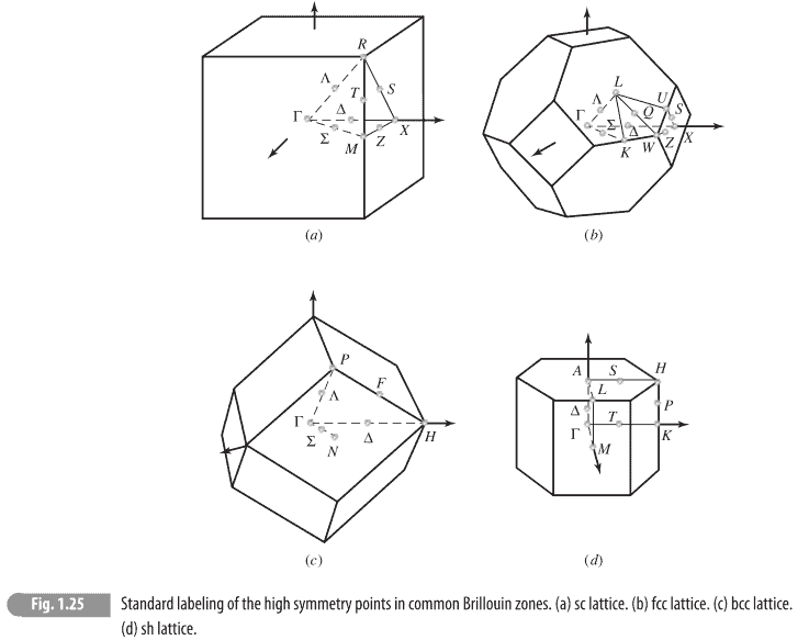
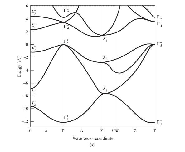
As discussed in Section 1.6, there are certain critical points in the Brillouin zone which correspond to the points on the surfaces of the zone that are half way between the origin and another reciprocal lattice vector. Figure 1.25 gives the standard labeling of these critical points for common lattice structures. Typically, band structure calculations give the band energies along lines from the center of the Brillouin zone to one of these points, or from one of these points to another one. Figure 1.26(a) shows a typical band structure plot for silicon, a cubic crystal. The critical points are labeled according to the drawing shown in Figure $1.25(\mathrm{~b})$. Note that the diagram is not symmetric about the $\Gamma$ point because two different paths away from this point are plotted. Note also that the $\mathrm{U} / \mathrm{K}$ point is not the midpoint between two reciprocal lattice points, and therefore the slope of the bands is not zero in every direction there; in particular, the slope is not zero along lines that are not normal to the zone boundary. The $\mathrm{L}$ and $\mathrm{X}$ points are critical points, and therefore if the bands are plotted with enough detail, one will see that they have zero slope at those points.
Figure 1.26(b) shows the density of states for the same crystal. As seen in this figure, van Hove singularities (discontinuities in the slope) correspond to critical points in the band structure. When bands overlap in energy, the density of states is just the sum of the density of states of the two bands. Notice that there is a gap in the density of states which corresponds to the energy gap in one band at the $\Gamma$ point (zone center) and the minimum of the next higher band at the $X$ point (the zone boundary in the [100] direction).

固体物理代写
物理代写|固体物理代写Solid-state physics代考|Electron Band Calculationsin Three Dimensions
到目前为止,我们已经研究了一个电子在固定外电位下的波函数。然而,在固体中,电子感受到的势能来自于每个电子与所有原子核和所有其他电子的相互作用。电子感受到的势能不仅是由带正电的原子核给出的,而且是由所有其他电子的平均负电荷给出的。
如果晶体具有一定的周期性,那么所有这些粒子形成的势也具有周期性,所以上面所有关于周期势的定理仍然适用。然而,确定电子带的确切性质是一项艰巨的任务。我们不能简单地解出固定势下单个电子的本征态;我们必须解出整个电子组的本征态,考虑到相同电子之间的交换,这必须根据费米统计来处理。处理电子费米统计量的方法将在第8章讨论。
一般来说,谱带结构的计算并不是一门精确的科学。通常,确定给定固体的能带结构涉及实验和理论之间的相互作用-通过x射线散射确定晶体对称性,计算能带结构,并通过其他实验如光吸收和反射率等进行校正。许多能带结构计算使用化学实验输入,如离子的电负性、键长等。从第一性原理计算能带结构,只使用原子核的电荷和质量,仍然是一个前沿研究领域,涉及高级数学和超级计算机。
在本书中,我们通常将电子带视为给定固体的已知函数。已经出版了许多实体的带图,并将其制成表格,例如《Madelung》(1996年)。同时,有几种有用的近似方法,使我们能够写出简单的带的数学公式,而不需要通过所有的计算来生成带结构。这些近似值并不能定量地预测实际的能带结构;相反,这些模型帮助我们对电子带的性质有了物理上的直观认识。
物理代写|固体物理代写Solid-state physics代考|How to Read a Band Diagram
在三维晶体中,所有能带能量的完整计算包括在三维布里渊带的每个点上找到每个能带的能量。这是大量的信息,我们需要以一种简单的方式来呈现它,以使其有用。
如1.6节所述,在布里渊区存在某些临界点,这些临界点对应于该区域表面上位于原点和另一个倒晶格向量中间的点。图1.25给出了常见晶格结构的这些临界点的标准标记。典型地,能带结构计算给出从布里渊带中心到其中一个点的能带能量,或者从其中一个点到另一个点的能带能量。图1.26(a)显示了立方体晶体硅的典型能带结构图。根据图$1.25(\ mathm {~b})$所示的绘图标记临界点。注意,该图对于$\Gamma$点不是对称的,因为从该点出发的两条不同路径被绘制出来。还要注意$\mathrm{U} / \mathrm{K}$点不是两个互反晶格点之间的中点,因此带的斜率在每个方向上都不是零;特别是,在不垂直于区域边界的直线上,斜率不为零。$\mathrm{L}$和$\mathrm{X}$点是临界点,因此,如果波段被绘制得足够详细,人们会看到它们在这些点上的斜率为零。
图1.26(b)显示了同一晶体的态密度。如图所示,van Hove奇点(斜率中的不连续点)对应于带结构中的临界点。当能带在能量上重叠时,态密度就是两个能带的态密度之和。请注意,态密度中存在一个缺口,对应于$\Gamma$点(区域中心)的一个能带的能量缺口,以及$X$点([100]方向的区域边界)的下一个更高能带的最小值。

统计代写请认准statistics-lab™. statistics-lab™为您的留学生涯保驾护航。
金融工程代写
金融工程是使用数学技术来解决金融问题。金融工程使用计算机科学、统计学、经济学和应用数学领域的工具和知识来解决当前的金融问题,以及设计新的和创新的金融产品。
非参数统计代写
非参数统计指的是一种统计方法,其中不假设数据来自于由少数参数决定的规定模型;这种模型的例子包括正态分布模型和线性回归模型。
广义线性模型代考
广义线性模型(GLM)归属统计学领域,是一种应用灵活的线性回归模型。该模型允许因变量的偏差分布有除了正态分布之外的其它分布。
术语 广义线性模型(GLM)通常是指给定连续和/或分类预测因素的连续响应变量的常规线性回归模型。它包括多元线性回归,以及方差分析和方差分析(仅含固定效应)。
有限元方法代写
有限元方法(FEM)是一种流行的方法,用于数值解决工程和数学建模中出现的微分方程。典型的问题领域包括结构分析、传热、流体流动、质量运输和电磁势等传统领域。
有限元是一种通用的数值方法,用于解决两个或三个空间变量的偏微分方程(即一些边界值问题)。为了解决一个问题,有限元将一个大系统细分为更小、更简单的部分,称为有限元。这是通过在空间维度上的特定空间离散化来实现的,它是通过构建对象的网格来实现的:用于求解的数值域,它有有限数量的点。边界值问题的有限元方法表述最终导致一个代数方程组。该方法在域上对未知函数进行逼近。[1] 然后将模拟这些有限元的简单方程组合成一个更大的方程系统,以模拟整个问题。然后,有限元通过变化微积分使相关的误差函数最小化来逼近一个解决方案。
tatistics-lab作为专业的留学生服务机构,多年来已为美国、英国、加拿大、澳洲等留学热门地的学生提供专业的学术服务,包括但不限于Essay代写,Assignment代写,Dissertation代写,Report代写,小组作业代写,Proposal代写,Paper代写,Presentation代写,计算机作业代写,论文修改和润色,网课代做,exam代考等等。写作范围涵盖高中,本科,研究生等海外留学全阶段,辐射金融,经济学,会计学,审计学,管理学等全球99%专业科目。写作团队既有专业英语母语作者,也有海外名校硕博留学生,每位写作老师都拥有过硬的语言能力,专业的学科背景和学术写作经验。我们承诺100%原创,100%专业,100%准时,100%满意。
随机分析代写
随机微积分是数学的一个分支,对随机过程进行操作。它允许为随机过程的积分定义一个关于随机过程的一致的积分理论。这个领域是由日本数学家伊藤清在第二次世界大战期间创建并开始的。
时间序列分析代写
随机过程,是依赖于参数的一组随机变量的全体,参数通常是时间。 随机变量是随机现象的数量表现,其时间序列是一组按照时间发生先后顺序进行排列的数据点序列。通常一组时间序列的时间间隔为一恒定值(如1秒,5分钟,12小时,7天,1年),因此时间序列可以作为离散时间数据进行分析处理。研究时间序列数据的意义在于现实中,往往需要研究某个事物其随时间发展变化的规律。这就需要通过研究该事物过去发展的历史记录,以得到其自身发展的规律。
回归分析代写
多元回归分析渐进(Multiple Regression Analysis Asymptotics)属于计量经济学领域,主要是一种数学上的统计分析方法,可以分析复杂情况下各影响因素的数学关系,在自然科学、社会和经济学等多个领域内应用广泛。
MATLAB代写
MATLAB 是一种用于技术计算的高性能语言。它将计算、可视化和编程集成在一个易于使用的环境中,其中问题和解决方案以熟悉的数学符号表示。典型用途包括:数学和计算算法开发建模、仿真和原型制作数据分析、探索和可视化科学和工程图形应用程序开发,包括图形用户界面构建MATLAB 是一个交互式系统,其基本数据元素是一个不需要维度的数组。这使您可以解决许多技术计算问题,尤其是那些具有矩阵和向量公式的问题,而只需用 C 或 Fortran 等标量非交互式语言编写程序所需的时间的一小部分。MATLAB 名称代表矩阵实验室。MATLAB 最初的编写目的是提供对由 LINPACK 和 EISPACK 项目开发的矩阵软件的轻松访问,这两个项目共同代表了矩阵计算软件的最新技术。MATLAB 经过多年的发展,得到了许多用户的投入。在大学环境中,它是数学、工程和科学入门和高级课程的标准教学工具。在工业领域,MATLAB 是高效研究、开发和分析的首选工具。MATLAB 具有一系列称为工具箱的特定于应用程序的解决方案。对于大多数 MATLAB 用户来说非常重要,工具箱允许您学习和应用专业技术。工具箱是 MATLAB 函数(M 文件)的综合集合,可扩展 MATLAB 环境以解决特定类别的问题。可用工具箱的领域包括信号处理、控制系统、神经网络、模糊逻辑、小波、仿真等。