如果你也在 怎样代写固体物理Solid-state physics这个学科遇到相关的难题，请随时右上角联系我们的24/7代写客服。

固态物理学是通过量子力学、晶体学、电磁学和冶金学等方法研究刚性物质或固体。它是凝聚态物理学的最大分支。

statistics-lab™ 为您的留学生涯保驾护航 在代写固体物理Solid-state physics方面已经树立了自己的口碑, 保证靠谱, 高质且原创的统计Statistics代写服务。我们的专家在代写固体物理Solid-state physics代写方面经验极为丰富，各种代写固体物理Solid-state physics相关的作业也就用不着说。

我们提供的固体物理Solid-state physics及其相关学科的代写，服务范围广, 其中包括但不限于:

• Statistical Inference 统计推断
• Statistical Computing 统计计算
• Advanced Probability Theory 高等概率论
• Advanced Mathematical Statistics 高等数理统计学
• (Generalized) Linear Models 广义线性模型
• Statistical Machine Learning 统计机器学习
• Longitudinal Data Analysis 纵向数据分析
• Foundations of Data Science 数据科学基础

物理代写|固体物理代写Solid-state physics代考|Boundary Conditions

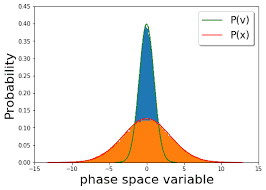
The wave function itself has no physical interpretation, however, the square of its absolute magnitude $|\Psi(x, t)|^2$ evaluated at a particular place and at a particular time is proportional to the possibility of finding the particle at that time. The probability density $|\Psi(x, t)|^2$ is positive and real and is taken equal to $\Psi^*(\boldsymbol{r}, t) \Psi(\boldsymbol{r}, t)$. The wave function $\Psi$ can take on negative values but probability density is always be positive. Besides fulfilling the normalization condition a solution of the time independent Schrödinger equation must obey the following boundary conditions.

1. The wave function must be continuous and single valued.
2. $\frac{\partial \psi}{\partial x}, \frac{\partial \psi}{\partial y}$ and $\frac{\partial \psi}{\partial z}$ must be continuous and single valued everywhere.
3. The integral of the square modulus of the wave function over all values $x$ must be finite
   $$
   \int \psi^* \psi \mathrm{d} \tau=\text { finite }
   $$
   that is the wave function must be square integrable. This condition means that wave function must be normalizable that is wave function must go to zero as $x(y, z) \rightarrow \pm \infty$ in order that $\int|\Psi|^2 \mathrm{~d} \tau$ over all space is finite constant.

The boundary conditions ensure that the probability of finding the particle in the vicinity of any point is unambiguously defined rather than having two or more possible values. Thus the wave function is single valued and continuous. If $\psi(x)$ and $(\mathrm{d} \psi / \mathrm{d} x)$ are not single valued, finite then the same is true for $\Psi(x, t)$. Since the given formula for calculating the expectation values of position and momentum contains $\Psi(x, t)$ and $\frac{\partial \Psi}{\partial t}$. We observe that in any of these cases we might not obtain finite and definite values when we evaluate measured quantities.

The first derivative of the wave function with respect to position coordinates must be continuous every where except where there is an infinite discontinuity in the potential. We know any function always has an infinite derivative whenever it has a discontinuity. Let us consider the time independent Schrödinger Eq. (4.67) in one dimension
$$
\frac{\mathrm{d}^2 \Psi}{\mathrm{d} x^2}=\frac{2 m}{\hbar^2}(V-E) \psi
$$
for finite $V, E$ and $\psi,\left(\mathrm{d}^2 \psi / \mathrm{d} x^2\right)$ is finite. This in turn requires (d $\psi / \mathrm{d} x$ ) to be continuous. A finite discontinuity in $(\mathrm{d} \psi / \mathrm{d} x)$ implies an infinite discontinuity in $\left(\mathrm{d}^2 \psi / \mathrm{d} x^2\right)$ and from the Schrödinger equation in $V(x)$.

物理代写|固体物理代写Solid-state physics代考|Hydrogen Atom

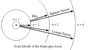
Consider the hydrogen atom as a system of two interacting particles, the interaction being due to Coulomb attraction of their electrical charges. Let the charge on the nucleus is $Z q$ and the charge on the electron is $-q$. The potential energy of the system in the absence of the external field is
$$
V(r)=-\frac{Z q^2}{\left(4 \pi \varepsilon_0\right) r}
$$
in which $r$ is the distance between the electron and the nucleus.
Let $m_1$ and $m_2$ are the masses of nucleus and the electron, respectively. If we write for the Cartesian coordinates of the nucleus and the electrons $x_1, y_1, z_1$ and $x_2, y_2, z_2$, respectively, the Hamiltonian of the hydrogenic atoms has the form
$$
H=\frac{p_1^2}{2 m_1}+\frac{p_2^2}{2 m_2}+V(r)=E
$$
The Schrödinger wave equation is $$
\frac{1}{m_1}\left(\frac{\partial^2 \Psi}{\partial x_1^2}+\frac{\partial^2 \Psi}{\partial y_1^2}+\frac{\partial^2 \Psi}{\partial z_1^2}\right)+\frac{1}{m_2}\left(\frac{\partial^2 \Psi}{\partial x_2^2}+\frac{\partial^2 \Psi}{\partial y_2^2}+\frac{\partial^2 \Psi}{\partial z_2^2}\right)+\frac{2}{\hbar^2}[E-V] \Psi=0
$$
Here wave function $\Psi$ refers to the complete system with six coordinates. Equation (4.73) can be separated into two, one of which represents the translational motion of a molecule as a whole and the other, the relative motion of the two particles. For this, consider new variables $X, Y, Z$ which are Cartesian coordinates of the centre of mass of the system and $r, \theta$ and $\varphi$ of the polar coordinates of the second particle relative to the first. These coordinates are related to the Cartesian coordinates of the two particles by the equations
$$
\begin{gathered}
X=\frac{m_1 x_1+m_2 x_2}{m_1+m_2} \
Y=\frac{m_1 y_1+m_2 y_2}{m_1+m_2} \
Z=\frac{m_1 z+m_2 z_2}{m_1+m_2} \
x=x_2-x_1=r \sin \theta \cos \varphi \
y=y_2-y_1=r \sin \theta \sin \varphi \
z=z_2-z_1=r \cos \theta
\end{gathered}
$$

固体物理代写

物理代写|固体物理代写Solid-state physics代考|Boundary Conditions

波函数本身没有物理解释，但是，它的绝对大小的平方 $|\Psi(x, t)|^2$ 在特定地点和特定时间评估的值与在该 时间找到粒子的可能性成正比。概率密度 $|\Psi(x, t)|^2$ 是正实数，取等于 $\Psi^*(\boldsymbol{r}, t) \Psi(\boldsymbol{r}, t)$. 波函数 $\Psi$ 可以 取负值，但概率密度始终为正。除了满足归一化条件外，与时间无关的薛定谔方程的解还必须遵守以下边 界条件。

1. 波函数必须是连续的和单值的。
2. $\frac{\partial \psi}{\partial x}, \frac{\partial \psi}{\partial y}$ 和 $\frac{\partial \psi}{\partial z}$ 必须是连续的并且处处都是单值的。
3. 波函数的平方模对所有值的积分 $x$ 必须是有限的
   $$
   \int \psi^* \psi \mathrm{d} \tau=\text { finite }
   $$
   即波函数必须是平方可积的。这个条件意味着波函数必须是可归一化的，即波函数必须归零为 $x(y, z) \rightarrow \pm \infty$ 为了使 $\int|\Psi|^2 \mathrm{~d} \tau$ 在所有空间上都是有限常数。
   边界条件确保在任何点附近找到粒子的概率被明确定义，而不是有两个或更多可能的值。因此波函数是单 值连续的。如果 $\psi(x)$ 和 $(\mathrm{d} \psi / \mathrm{d} x)$ 不是单值的，有限的那么同样适用于 $\Psi(x, t)$. 由于用于计算位置和动 量期望值的给定公式包含 $\Psi(x, t)$ 和 $\frac{\partial \Psi}{\partial t}$. 我们观察到，在任何这些情况下，当我们评估测量量时，我们可 能无法获得有限和确定的值。
   波函数相对于位置坐标的一阶导数在任何地方都必须是连续的，除了势能中存在无限不连续的地方。我们 知道，任何函数只要有不连续点，就总是有无穷导数。让我们考虑时间无关的薛定谔方程。(4.67) 一维
   $$
   \frac{\mathrm{d}^2 \Psi}{\mathrm{d} x^2}=\frac{2 m}{\hbar^2}(V-E) \psi
   $$
   对于有限 $V, E$ 和 $\psi,\left(\mathrm{d}^2 \psi / \mathrm{d} x^2\right)$ 是有限的。这又需要 $(\mathrm{d} \psi / \mathrm{d} x)$ 是连续的。中的有限不连续性 $(\mathrm{d} \psi / \mathrm{d} x)$ 意味着无限不连续 $\left(\mathrm{d}^2 \psi / \mathrm{d} x^2\right)$ 从薛定谔方程 $V(x)$.

物理代写|固体物理代写Solid-state physics代考|Hydrogen Atom

将氢原子视为两个相互作用粒子的系统，相互作用是由于它们的电荷的库仑吸引。让原子核上的电荷是 $Z q$ 电子上的电荷是 $-q$. 在没有外场的情况下系统的势能是
$$
V(r)=-\frac{Z q^2}{\left(4 \pi \varepsilon_0\right) r}
$$
其中 $r$ 是电子与原子核之间的距离。
让 $m_1$ 和 $m_2$ 分别是原子核和电子的质量。如果我们写下原子核和电子的笛卡尔坐标 $x_1, y_1, z_1$ 和 $x_2, y_2, z_2$ ，氢原子的哈密顿量分别具有以下形式
$$
H=\frac{p_1^2}{2 m_1}+\frac{p_2^2}{2 m_2}+V(r)=E
$$
辠定谔波动方程是
$$
\frac{1}{m_1}\left(\frac{\partial^2 \Psi}{\partial x_1^2}+\frac{\partial^2 \Psi}{\partial y_1^2}+\frac{\partial^2 \Psi}{\partial z_1^2}\right)+\frac{1}{m_2}\left(\frac{\partial^2 \Psi}{\partial x_2^2}+\frac{\partial^2 \Psi}{\partial y_2^2}+\frac{\partial^2 \Psi}{\partial z_2^2}\right)+\frac{2}{\hbar^2}[E-V] \Psi=0
$$
这里的波函数 $\Psi$ 指具有六个坐标的完整系统。方程 (4.73) 可以分为两个，一个表示分子整体的平移运 动，另一个表示两个粒子的相对运动。为此，考虑新变量 $X, Y, Z$ 这是系统质心的笛卡尔坐标和 $r, \theta$ 和 $\varphi$ 第二个粒子相对于第一个粒子的极坐标。这些坐标通过方程式与两个粒子的笛卡尔坐标相关
$$
X=\frac{m_1 x_1+m_2 x_2}{m_1+m_2} Y=\frac{m_1 y_1+m_2 y_2}{m_1+m_2} Z=\frac{m_1 z+m_2 z_2}{m_1+m_2} x=x_2-x_1=r \sin \theta \cos \varphi y=y_2
$$

统计代写请认准statistics-lab™. statistics-lab™为您的留学生涯保驾护航。

金融工程代写

金融工程是使用数学技术来解决金融问题。金融工程使用计算机科学、统计学、经济学和应用数学领域的工具和知识来解决当前的金融问题，以及设计新的和创新的金融产品。

非参数统计代写

非参数统计指的是一种统计方法，其中不假设数据来自于由少数参数决定的规定模型；这种模型的例子包括正态分布模型和线性回归模型。

广义线性模型代考

广义线性模型（GLM）归属统计学领域，是一种应用灵活的线性回归模型。该模型允许因变量的偏差分布有除了正态分布之外的其它分布。

术语 广义线性模型（GLM）通常是指给定连续和/或分类预测因素的连续响应变量的常规线性回归模型。它包括多元线性回归，以及方差分析和方差分析（仅含固定效应）。

有限元方法代写

有限元方法（FEM）是一种流行的方法，用于数值解决工程和数学建模中出现的微分方程。典型的问题领域包括结构分析、传热、流体流动、质量运输和电磁势等传统领域。

有限元是一种通用的数值方法，用于解决两个或三个空间变量的偏微分方程（即一些边界值问题）。为了解决一个问题，有限元将一个大系统细分为更小、更简单的部分，称为有限元。这是通过在空间维度上的特定空间离散化来实现的，它是通过构建对象的网格来实现的：用于求解的数值域，它有有限数量的点。边界值问题的有限元方法表述最终导致一个代数方程组。该方法在域上对未知函数进行逼近。[1] 然后将模拟这些有限元的简单方程组合成一个更大的方程系统，以模拟整个问题。然后，有限元通过变化微积分使相关的误差函数最小化来逼近一个解决方案。

tatistics-lab作为专业的留学生服务机构，多年来已为美国、英国、加拿大、澳洲等留学热门地的学生提供专业的学术服务，包括但不限于Essay代写，Assignment代写，Dissertation代写，Report代写，小组作业代写，Proposal代写，Paper代写，Presentation代写，计算机作业代写，论文修改和润色，网课代做，exam代考等等。写作范围涵盖高中，本科，研究生等海外留学全阶段，辐射金融，经济学，会计学，审计学，管理学等全球99%专业科目。写作团队既有专业英语母语作者，也有海外名校硕博留学生，每位写作老师都拥有过硬的语言能力，专业的学科背景和学术写作经验。我们承诺100%原创，100%专业，100%准时，100%满意。

随机分析代写

随机微积分是数学的一个分支，对随机过程进行操作。它允许为随机过程的积分定义一个关于随机过程的一致的积分理论。这个领域是由日本数学家伊藤清在第二次世界大战期间创建并开始的。

时间序列分析代写

随机过程，是依赖于参数的一组随机变量的全体，参数通常是时间。 随机变量是随机现象的数量表现，其时间序列是一组按照时间发生先后顺序进行排列的数据点序列。通常一组时间序列的时间间隔为一恒定值（如1秒，5分钟，12小时，7天，1年），因此时间序列可以作为离散时间数据进行分析处理。研究时间序列数据的意义在于现实中，往往需要研究某个事物其随时间发展变化的规律。这就需要通过研究该事物过去发展的历史记录，以得到其自身发展的规律。

回归分析代写

多元回归分析渐进（Multiple Regression Analysis Asymptotics）属于计量经济学领域，主要是一种数学上的统计分析方法，可以分析复杂情况下各影响因素的数学关系，在自然科学、社会和经济学等多个领域内应用广泛。

MATLAB代写

MATLAB 是一种用于技术计算的高性能语言。它将计算、可视化和编程集成在一个易于使用的环境中，其中问题和解决方案以熟悉的数学符号表示。典型用途包括：数学和计算算法开发建模、仿真和原型制作数据分析、探索和可视化科学和工程图形应用程序开发，包括图形用户界面构建MATLAB 是一个交互式系统，其基本数据元素是一个不需要维度的数组。这使您可以解决许多技术计算问题，尤其是那些具有矩阵和向量公式的问题，而只需用 C 或 Fortran 等标量非交互式语言编写程序所需的时间的一小部分。MATLAB 名称代表矩阵实验室。MATLAB 最初的编写目的是提供对由 LINPACK 和 EISPACK 项目开发的矩阵软件的轻松访问，这两个项目共同代表了矩阵计算软件的最新技术。MATLAB 经过多年的发展，得到了许多用户的投入。在大学环境中，它是数学、工程和科学入门和高级课程的标准教学工具。在工业领域，MATLAB 是高效研究、开发和分析的首选工具。MATLAB 具有一系列称为工具箱的特定于应用程序的解决方案。对于大多数 MATLAB 用户来说非常重要，工具箱允许您学习和应用专业技术。工具箱是 MATLAB 函数（M 文件）的综合集合，可扩展 MATLAB 环境以解决特定类别的问题。可用工具箱的领域包括信号处理、控制系统、神经网络、模糊逻辑、小波、仿真等。

如果你也在 怎样代写固体物理Solid-state physics这个学科遇到相关的难题，请随时右上角联系我们的24/7代写客服。

固态物理学是通过量子力学、晶体学、电磁学和冶金学等方法研究刚性物质或固体。它是凝聚态物理学的最大分支。

statistics-lab™ 为您的留学生涯保驾护航 在代写固体物理Solid-state physics方面已经树立了自己的口碑, 保证靠谱, 高质且原创的统计Statistics代写服务。我们的专家在代写固体物理Solid-state physics代写方面经验极为丰富，各种代写固体物理Solid-state physics相关的作业也就用不着说。

我们提供的固体物理Solid-state physics及其相关学科的代写，服务范围广, 其中包括但不限于:

• Statistical Inference 统计推断
• Statistical Computing 统计计算
• Advanced Probability Theory 高等概率论
• Advanced Mathematical Statistics 高等数理统计学
• (Generalized) Linear Models 广义线性模型
• Statistical Machine Learning 统计机器学习
• Longitudinal Data Analysis 纵向数据分析
• Foundations of Data Science 数据科学基础

物理代写|固体物理代写Solid-state physics代考|Parabolic bands approximation

If we concentrate on considering only the band portions close to the VB top and the CB bottom, we recognise that in these regions the bands have a trend that, in very good approximation, can be described as parabolic (see figures $8.7$ and $8.8$ at the $\Gamma$ point). Therefore, whenever we are interested in studying the physics of electrons in the proximity of the forbidden gap, we can meaningfully use the so called parabolic bands approximation.

This approximation is straightforwardly applied in the one-dimensional case by taking the limit of $k \rightarrow 0$ of equations (8.20) and (8.21)
$$
\begin{aligned}
& \lim {k \rightarrow 0} E{\mathrm{VB}}(k)=E_{\mathrm{a}}+2 \gamma\left[1-\frac{(k a)^2}{2}\right] \
& \lim {k \rightarrow 0} E{\mathrm{CB}}(k)=E_{\mathrm{a}}^{\prime}-2 \delta\left[1-\frac{(k a)^2}{2}\right] .
\end{aligned}
$$
Taking this limit is justified by the fact that at $k=0$ we found both the VB top and the CB bottom, as shown in figure 8.6. A general remarkable feature is drawn: the thermal excitation of electrons basically occurs within a parabolic band scheme.

It is very convenient to address electron dynamics within a semi-classical scheme according to which: (i) electron energy states are described quantum mechanically,but (ii) their equations of motion are classical. This approximated scheme is trustworthy when one wants to study the motion of the electrons over a length scale much larger than the interatomic distances. This is, for instance, the relevant case of motion under the action of an externally applied and slowly varying electric field, that is an electric field which is practically constant over the length scale of interatomic lattice distances. On the other hand, the results of this approximation can hardly be extended to the case of nanostructures [16, 17], that is to solid state systems whose structural features display on the $10^{-9} \mathrm{~m}$ scale: here a full quantum theory of electron transport is needed, as detailed elsewhere [12, 17-19].

物理代写|固体物理代写Solid-state physics代考|Electric field effects

Let us now apply a constant and uniform electric field $\mathbf{E}$ along a one-dimensional crystal. Within the semi-classical scheme a driving force
$$
F=-e|\mathbf{E}|=\hbar \frac{d k}{d t},
$$
is calculated, governing the drift motion of the electron. The solution of this equation of motion is
$$
k(t)=k_0-\frac{e|\mathbf{E}|}{\hbar} t,
$$
where $k_0$ is the electron wavevector at time $t=0$, that is, when the electric field is turned on. By making use of equation (8.29) this result reflects in a time-dependent electron velocity
$$
v_n(k, t)=\frac{1}{\hbar} \frac{d E_n}{d k(t)}
$$

suggesting the practical rule that under the action of an electric field, the electron velocity at time $t$ is calculated by evaluating the slope of band tangent at the point $k(t)$ given in equation (8.32). This result has a quite interesting implication, as we easily understand by considering the case of an electron in the valence band: under the action of the electric field, which we consider oriented to the left with no loss of generality, the wavevector varies linearly with time, assuming gradually increasing values and, therefore, it will sooner or later end up reaching the right edge of the 1BL. However, given the crystalline periodicity, the $k=+\pi / a$ value defines a quantum state equivalent to the one described by $k^{\prime}=k+G$ with $G=-2 \pi / a$ a reciprocal lattice vector. This is tantamount to saying that the electron, once it reaches the right edge, is flipped back to a state corresponding the left one. Next, as time goes by, the electron will again assume increasing wavevector values, as before eventually reaching the right edge of $1 \mathrm{BZ}$ : here its wavevector will be flipped back once more. And so on … This periodic back-and-forth variation of $k(t)$ in the Brillouin zone will continue as long as the electric field is present. This phenomenon is described by saying that under the action of an electric field a band electron is subjected to Bloch oscillations: their graphical rendering is reported in figure $8.10$.
We remark that this result has been obtained by guessing the equation of motion (8.31) where no scattering phenomena appear, contrarily to what we discussed in section 7.1. This is of course a very crude approximation: in practice, it is very difficult to experimentally observe Bloch oscillations in real materials just because ionic motions and defects disturb the electron motion. Such oscillations are only detected at low temperature and in chemically pure systems, since the occurrence of such circumstances makes the periodic variation of $k(t)$ only marginally affected by electron-phonon and electron-defect scattering events or, equivalently, the friction term appearing in equation (7.3) to play a marginal role.

固体物理代写

物理代写|固体物理代写Solid-state physics代考|Parabolic bands approximation

如果我们只专注于考虑靠近 VB 顶部和 CB 底部的波段部分，我们会认识到在这些区域中，波 段有一个趋势，在非常近似的情况下，可以描述为抛物线 (见图 $8.7$ 和 $8.8$ 在 $\Gamma$ 观点) 。因此， 每当我们有兴趣研究禁带附近的电子物理时，我们都可以有意义地使用所谓的抛物线近似。
该近似值直接应用于一维情况，取的极限是 $k \rightarrow 0$ 等式 (8.20) 和 (8.21)
$$
\lim k \rightarrow 0 E \operatorname{VB}(k)=E_{\mathrm{a}}+2 \gamma\left[1-\frac{(k a)^2}{2}\right] \quad \lim k \rightarrow 0 E \operatorname{CB}(k)=E_{\mathrm{a}}^{\prime}-2 \delta[1
$$
采取这个限制是合理的，因为在 $k=0$ 我们找到了 $\mathrm{VB}$ 顶部和 $\mathrm{CB}$ 底部，如图 $8.6$ 所示。得出一 个普㴜的显着特征: 电子的热激发基本上发生在抛物线带方案内。
在半经典方案中解决电子动力学非常方便，根据该方案: (i) 电子能态用量子力学描述，但 (ii) 它们的运动方程是经典的。当人们想要研究电子在比原子间距离大得多的长度尺度上的运动 时，这种近似方案是值得信赖的。例如，这是在外部施加的缓曼变化的电场作用下运动的相关 情况，该电场在原子间晶格距离的长度尺度上实际上是恒定的。另一方面，这种近似的结果很 难扩展到纳米结构的情况 [16，17]，即结构特征显示在 $10^{-9} \mathrm{~m}$ 规模: 这里需要一个完整的电 子传输量子理论，正如其他地方详述的那样 [12, 17-19]。

物理代写|固体物理代写Solid-state physics代考|Electric field effects

现在让我们施加一个恒定且均匀的电场E沿着一维晶体。在半经典方案中，驱动力
$$
F=-e|\mathbf{E}|=\hbar \frac{d k}{d t},
$$
计算，控制电子的漂移运动。这个运动方程的解是
$$
k(t)=k_0-\frac{e|\mathbf{E}|}{\hbar} t
$$
在哪里 $k_0$ 是时刻的电子波矢 $t=0$ ，也就是说，当电场打开时。通过使用等式 (8.29)，该结果 反映在时间相关的电子速度中
$$
v_n(k, t)=\frac{1}{\hbar} \frac{d E_n}{d k(t)}
$$
表明在电场作用下，电子速度随时间变化的实际规律 $t$ 通过评估带切线在该点的斜率来计算 $k(t)$ 在等式 (8.32) 中给出。这个结果有一个非常有趣的含义，正如我们通过考虑价带中电子的 情况很容易理解的那样: 在不失一般性的情况下我们认为向左取向的电场的作用下，波矢量线 性变化时间，假设值逐渐增加，因此迟早会到达 1BL 的右边缘。然而，考虑到晶体的周期性， $k=+\pi / a$ value 定义了一个量子态，等价于由 $k^{\prime}=k+G$ 和 $G=-2 \pi / a$ 倒数点阵向量。 这无异于说电子一旦到达右边缘，就会翻转回与左边缘对应的状态。接下来，随着时间的流 逝，电子将再次呈现增加的波矢值，就像之前最终到达右边缘一样 $1 \mathrm{BZ}$ ：这里它的波向量将再 次翻转回来。依此类推……这种周期性的来回变化 $k(t)$ 只要存在电场，布里渊区的光就会继 续。这种现象的描述是，在电扬的作用下，带电子受到布洛赫振荡：它们的图形洹染如图所示 $8.10$.
我们注意到这个结果是通过猜测没有出现散射现象的运动方程 (8.31) 获得的，这与我们在 $7.1$ 节中讨论的相反。这当然是一个非常粗略的近似值：在实践中，很难仅仅因为离子运动和缺陷 干扰电子运动而通过实验观察真实材料中的布洛赫振荡。这种振荡仅在低温和化学纯系统中检 测到，因为这种情况的发生使得 $k(t)$ 仅受电子声子和电子缺陷散射事件的轻微影响，或者等效 地，等式 (7.3) 中出现的摩擦项起着微不足道的作用。

统计代写请认准statistics-lab™. statistics-lab™为您的留学生涯保驾护航。

金融工程代写

金融工程是使用数学技术来解决金融问题。金融工程使用计算机科学、统计学、经济学和应用数学领域的工具和知识来解决当前的金融问题，以及设计新的和创新的金融产品。

非参数统计代写

非参数统计指的是一种统计方法，其中不假设数据来自于由少数参数决定的规定模型；这种模型的例子包括正态分布模型和线性回归模型。

广义线性模型代考

广义线性模型（GLM）归属统计学领域，是一种应用灵活的线性回归模型。该模型允许因变量的偏差分布有除了正态分布之外的其它分布。

术语 广义线性模型（GLM）通常是指给定连续和/或分类预测因素的连续响应变量的常规线性回归模型。它包括多元线性回归，以及方差分析和方差分析（仅含固定效应）。

有限元方法代写

有限元方法（FEM）是一种流行的方法，用于数值解决工程和数学建模中出现的微分方程。典型的问题领域包括结构分析、传热、流体流动、质量运输和电磁势等传统领域。

有限元是一种通用的数值方法，用于解决两个或三个空间变量的偏微分方程（即一些边界值问题）。为了解决一个问题，有限元将一个大系统细分为更小、更简单的部分，称为有限元。这是通过在空间维度上的特定空间离散化来实现的，它是通过构建对象的网格来实现的：用于求解的数值域，它有有限数量的点。边界值问题的有限元方法表述最终导致一个代数方程组。该方法在域上对未知函数进行逼近。[1] 然后将模拟这些有限元的简单方程组合成一个更大的方程系统，以模拟整个问题。然后，有限元通过变化微积分使相关的误差函数最小化来逼近一个解决方案。

tatistics-lab作为专业的留学生服务机构，多年来已为美国、英国、加拿大、澳洲等留学热门地的学生提供专业的学术服务，包括但不限于Essay代写，Assignment代写，Dissertation代写，Report代写，小组作业代写，Proposal代写，Paper代写，Presentation代写，计算机作业代写，论文修改和润色，网课代做，exam代考等等。写作范围涵盖高中，本科，研究生等海外留学全阶段，辐射金融，经济学，会计学，审计学，管理学等全球99%专业科目。写作团队既有专业英语母语作者，也有海外名校硕博留学生，每位写作老师都拥有过硬的语言能力，专业的学科背景和学术写作经验。我们承诺100%原创，100%专业，100%准时，100%满意。

随机分析代写

随机微积分是数学的一个分支，对随机过程进行操作。它允许为随机过程的积分定义一个关于随机过程的一致的积分理论。这个领域是由日本数学家伊藤清在第二次世界大战期间创建并开始的。

时间序列分析代写

随机过程，是依赖于参数的一组随机变量的全体，参数通常是时间。 随机变量是随机现象的数量表现，其时间序列是一组按照时间发生先后顺序进行排列的数据点序列。通常一组时间序列的时间间隔为一恒定值（如1秒，5分钟，12小时，7天，1年），因此时间序列可以作为离散时间数据进行分析处理。研究时间序列数据的意义在于现实中，往往需要研究某个事物其随时间发展变化的规律。这就需要通过研究该事物过去发展的历史记录，以得到其自身发展的规律。

回归分析代写

多元回归分析渐进（Multiple Regression Analysis Asymptotics）属于计量经济学领域，主要是一种数学上的统计分析方法，可以分析复杂情况下各影响因素的数学关系，在自然科学、社会和经济学等多个领域内应用广泛。

MATLAB代写

MATLAB 是一种用于技术计算的高性能语言。它将计算、可视化和编程集成在一个易于使用的环境中，其中问题和解决方案以熟悉的数学符号表示。典型用途包括：数学和计算算法开发建模、仿真和原型制作数据分析、探索和可视化科学和工程图形应用程序开发，包括图形用户界面构建MATLAB 是一个交互式系统，其基本数据元素是一个不需要维度的数组。这使您可以解决许多技术计算问题，尤其是那些具有矩阵和向量公式的问题，而只需用 C 或 Fortran 等标量非交互式语言编写程序所需的时间的一小部分。MATLAB 名称代表矩阵实验室。MATLAB 最初的编写目的是提供对由 LINPACK 和 EISPACK 项目开发的矩阵软件的轻松访问，这两个项目共同代表了矩阵计算软件的最新技术。MATLAB 经过多年的发展，得到了许多用户的投入。在大学环境中，它是数学、工程和科学入门和高级课程的标准教学工具。在工业领域，MATLAB 是高效研究、开发和分析的首选工具。MATLAB 具有一系列称为工具箱的特定于应用程序的解决方案。对于大多数 MATLAB 用户来说非常重要，工具箱允许您学习和应用专业技术。工具箱是 MATLAB 函数（M 文件）的综合集合，可扩展 MATLAB 环境以解决特定类别的问题。可用工具箱的领域包括信号处理、控制系统、神经网络、模糊逻辑、小波、仿真等。

如果你也在 怎样代写固体物理Solid-state physics这个学科遇到相关的难题，请随时右上角联系我们的24/7代写客服。

固态物理学是通过量子力学、晶体学、电磁学和冶金学等方法研究刚性物质或固体。它是凝聚态物理学的最大分支。

statistics-lab™ 为您的留学生涯保驾护航 在代写固体物理Solid-state physics方面已经树立了自己的口碑, 保证靠谱, 高质且原创的统计Statistics代写服务。我们的专家在代写固体物理Solid-state physics代写方面经验极为丰富，各种代写固体物理Solid-state physics相关的作业也就用不着说。

我们提供的固体物理Solid-state physics及其相关学科的代写，服务范围广, 其中包括但不限于:

• Statistical Inference 统计推断
• Statistical Computing 统计计算
• Advanced Probability Theory 高等概率论
• Advanced Mathematical Statistics 高等数理统计学
• (Generalized) Linear Models 广义线性模型
• Statistical Machine Learning 统计机器学习
• Longitudinal Data Analysis 纵向数据分析
• Foundations of Data Science 数据科学基础

物理代写|固体物理代写Solid-state physics代考|Bands in a one-dimensional crystal

Let us consider a monoatomic linear chain of atoms with lattice spacing $a$ so that ion positions are given by $x_s=s a$ with $s=0, \pm 1, \pm 2, \pm 3, \ldots$. Let us also suppose that there is just one valence electron for each atom in the chain. The Born-von Karman boundary condition given in equation (1.4) is applied to a crystal portion containing a suitably large number $N$ of atoms (and, therefore an equal number $N_{\text {val }}=N$ of valence electrons).

The preliminary step in our approach is to consider the case of a single isolated atom of the same chemical species present in the chain. Let $\hat{V}{\mathrm{a}}$ be the quantum operator describing the potential $V{\mathrm{a}}$ felt by the valence electron and let us suppose that the corresponding Schrödinger problem
$$
\left[-\frac{\hbar^2}{2 m} \nabla^2+\hat{V}{\mathrm{a}}\right] \phi{\mathrm{a}}=E_{\mathrm{a}} \phi_{\mathrm{a}}
$$
has been solved by means of the standard methods of atomic physics [7-9]. In our formalism $\phi_{\mathrm{a}}$ e $E_{\mathrm{a}}$ are the atomic wavefunction and energy of the atomic states, respectively.

Once the atom is placed in some lattice position along the chain, we can assume to a very good approximation that its valence electron is now subject to a potential $V_{\mathrm{c}}(x)$ written $\mathrm{as}^5$
$$
V_{\mathrm{c}}(x)=V_{\mathrm{a}}+\Delta V(x)
$$
where $\Delta V(x)$ describes the difference between the crystalline environment and the isolated atom situation. Our physical intuition suggests that $\Delta V(x)$ is vanishingly small in the core regions, while it significantly differs from zero in the interstitial ones, as qualitatively reported in figure 6.3. Obviously $\Delta V(x)=\Delta V(x+s a)$. The crystalline Schrödinger problem is therefore written as
$$
\left[-\frac{\hbar^2}{2 m} \frac{d^2}{d x^2}+\hat{V}{\mathrm{c}}(x)\right] \psi{\mathrm{c}}(x)=E_{\mathrm{c}} \psi_{\mathrm{c}}(x),
$$
where $\hat{V}{\mathrm{c}}(x)$ is the quantum operator corresponding to the potential given in equation (8.8), while $\psi{\mathrm{c}}(x)$ and $E_{\mathrm{c}}$ are the wavefunction and energy of the crystalline states, respectively. For further convenience, we recast this equation in a more compact form
$$
\hat{H} \psi_{\mathrm{c}}(x)=E_{\mathrm{c}} \psi_{\mathrm{c}}(x) \quad \text { where } \quad \hat{H}=-\frac{\hbar^2}{2 m} \frac{d^2}{d x^2}+\hat{V}_{\mathrm{c}}(x)
$$

物理代写|固体物理代写Solid-state physics代考|Bands in real solids

The tight-binding theory can also be applied to three-dimensional solids $[1,10,12,13]$ in any possible crystal structure or chemical composition, as well as containing an arbitrary number of valence electrons. Although the theory is developed in the same way as described in the previous section, the resulting mathematics is definitely more complicated, as shown in full detail in appendix $G$ : here we simply outline the procedure from a conceptual point of view and discuss a few paradigmatic applications.

The starting point is to write the crystalline wavefunction in a $\mathrm{LCAO}$ form by using a set of suitable localised orbitals $\left{\varphi_{a \mathrm{lb}}(\mathbf{r})=\varphi_\alpha\left(\mathbf{r}-\mathbf{R}1-\mathbf{R}{\mathrm{b}}\right)\right}$ centred on the different ion positions ${ }^8$; the label $\alpha$ stands for the full set of quantum numbers defining the corresponding state. In principle, such orbitals can be true atomic wavefunctions which, however, form a non-orthogonal basis set since orbitals centred on different lattice positions are not so; alternatively, an orthogonalisation procedure can be operated, as detailed in appendix $\mathrm{G}$, still preserving the $s^{-}, p-, d-, \cdots$ character of the atomic orbitals.

In order to set up a formalism naturally obeying the Bloch theorem, the following Bloch sums are defined
$$
\varphi_{a b \mathbf{k}}^{\mathrm{Bloch}}(\mathbf{r})=\frac{1}{\sqrt{N}} \sum_1 \mathrm{e}^{i \mathbf{k} \cdot \mathbf{R}1} \varphi_a\left(\mathbf{r}-\mathbf{R}_1-\mathbf{R}{\mathrm{b}}\right),
$$
where $N$ is the number of unit cells contained in the crystal portion subject to the periodic Born-von Karman boundary condition. The electron wavefunction for the $n$th band is accordingly cast in the following LCAO form
$$
\begin{aligned}
& =\frac{1}{\sqrt{N N_{\mathrm{b}}}} \sum_{a \mathrm{lb}} B_{n a \mathrm{~b}}(\mathbf{k}) \varphi_a\left(\mathbf{r}-\mathbf{R}1-\mathbf{R}{\mathrm{b}}\right), \
&
\end{aligned}
$$
where $N_{\mathrm{b}}$ is the number of atoms in the lattice basis, $\tilde{B}{n a \mathrm{~b}}$ are the LCAO expansion coefficients, and for brevity we have set $B{n a l b}(\mathbf{k})=\exp \left(i \mathbf{k} \cdot \mathbf{R}1\right) \tilde{B}{n a \mathrm{~b}}$.

固体物理代写

物理代写|固体物理代写Solid-state physics代考|Bands in a one-dimensional crystal

让我们考虑具有晶格间距的单原子线性原子链 $a$ 离子位置由下式给出 $x_s=s a$ 和 $s=0, \pm 1, \pm 2, \pm 3, \ldots$. 我们还假设链中每个原子只有一个价电子。等式 (1.4) 中给出的 Born-von Karman 边界条件应用于包含适当大数的晶体部分 $N$ 原子 (因此，数量相等 $N_{\mathrm{val}}=N$ 价电子) 。
我们方法的第一步是考虑链中存在的相同化学物质的单个孤立原子的情况。让 $\hat{V} \mathrm{a}$ 是描述势能 的量子算子 $V$ a被价电子感觉到，让我们假设相应的薛定谔问题
$$
\left[-\frac{\hbar^2}{2 m} \nabla^2+\hat{V} \mathrm{a}\right] \phi \mathrm{a}=E_{\mathrm{a}} \phi_{\mathrm{a}}
$$
已经通过原子物理学的标准方法解决了[7-9]。在我们的形式主义中 $\phi_{\mathrm{a}}$ 这是 $E_{\mathrm{a}}$ 分别是原子态的 原子波函数和能量。
一旦原子被放置在链上的某个晶格位置，我们可以非常近似地假设它的价电子现在受到势能的 影响 $V_{\mathrm{c}}(x)$ 书面 $\mathrm{as}^5$
$$
V_{\mathrm{c}}(x)=V_{\mathrm{a}}+\Delta V(x)
$$
在哪里 $\Delta V(x)$ 描述了晶体环境和孤立原子情况之间的差异。我们的物理直觉表明 $\Delta V(x)$ 如图 $6.3$ 中定性报告的那样，在核心区域中小得几乎消失，而在间隙区域中它与零有显着差异。明 显地 $\Delta V(x)=\Delta V(x+s a)$. 因此，晶体薛定谔问题被写为
$$
\left[-\frac{\hbar^2}{2 m} \frac{d^2}{d x^2}+\hat{V} \mathrm{c}(x)\right] \psi \mathrm{c}(x)=E_{\mathrm{c}} \psi_{\mathrm{c}}(x),
$$
在哪里 $\hat{V} \mathrm{c}(x)$ 是对应于等式 (8.8) 中给出的势的量子算符，而 $\psi \mathrm{c}(x)$ 和 $E_{\mathrm{c}}$ 分别是晶态的波函数 和能量。为了进一步方便，我们以更紧凑的形式重写这个等式
$$
\hat{H} \psi_{\mathrm{c}}(x)=E_{\mathrm{c}} \psi_{\mathrm{c}}(x) \quad \text { where } \quad \hat{H}=-\frac{\hbar^2}{2 m} \frac{d^2}{d x^2}+\hat{V}_{\mathrm{c}}(x)
$$

物理代写|固体物理代写Solid-state physics代考|Bands in real solids

紧

紧束缚理论也可以应用于三维固体 $[1,10,12,13]$ 在任何可能的晶体结构或化学组成中，以及 包含任意数量的价电子。尽管该理论的发展方式与上一节所述相同，但由此产生的数学肯定更 加复杂，如附录中的详细信息所示 $G$ : 在这里，我们只是从概念的角度概述了该过程，并讨论 了一些范例应用程序。
起点是将晶体波函数写成LCAO通过使用一组合适的局部轨道形成
以不同的离子位置为中心 ${ }^8$; 标签 $\alpha$ 代表定义相应状态的全套量子数。原则上，这样的轨道可以 是真正的原子波函数，然而，由于以不同晶格位置为中心的轨道并非如此，因此形成非正交基 组；或者，可以运行正交化程序，详见附录G，仍然保留 $s^{-}, p-, d-, \cdots$ 原子轨道的性质。
为了建立自然服从布洛赫定理的形式主义，定义了以下布洛赫和
$$
\varphi_{a b \mathbf{k}}^{\text {Bloch }}(\mathbf{r})=\frac{1}{\sqrt{N}} \sum_1 \mathrm{e}^{i \mathbf{k} \cdot \mathbf{R} 1} \varphi_a\left(\mathbf{r}-\mathbf{R}1-\mathbf{R b}\right), $$ 在哪里 $N$ 是受周期性 Born-von Karman 边界条件影响的晶体部分中包含的晶怉数。电子波函 数为 $n$th 频段相应地采用以下 LCAO 形式 $$ =\frac{1}{\sqrt{N N{\mathrm{b}}}} \sum_{a \mathrm{lb}} B_{n a \mathrm{~b}}(\mathbf{k}) \varphi_a(\mathbf{r}-\mathbf{R} 1-\mathbf{R b}),
$$
在哪里 $N_{\mathrm{b}}$ 是晶格基中的原子数， $\tilde{B} n a \mathrm{~b}$ 是 LCAO 扩展系数，为了简洁起见，我们设置了 $\operatorname{Bnalb}(\mathbf{k})=\exp (i \mathbf{k} \cdot \mathbf{R} 1) \tilde{B} n a$ b

统计代写请认准statistics-lab™. statistics-lab™为您的留学生涯保驾护航。

金融工程代写

金融工程是使用数学技术来解决金融问题。金融工程使用计算机科学、统计学、经济学和应用数学领域的工具和知识来解决当前的金融问题，以及设计新的和创新的金融产品。

非参数统计代写

非参数统计指的是一种统计方法，其中不假设数据来自于由少数参数决定的规定模型；这种模型的例子包括正态分布模型和线性回归模型。

广义线性模型代考

广义线性模型（GLM）归属统计学领域，是一种应用灵活的线性回归模型。该模型允许因变量的偏差分布有除了正态分布之外的其它分布。

术语 广义线性模型（GLM）通常是指给定连续和/或分类预测因素的连续响应变量的常规线性回归模型。它包括多元线性回归，以及方差分析和方差分析（仅含固定效应）。

有限元方法代写

有限元方法（FEM）是一种流行的方法，用于数值解决工程和数学建模中出现的微分方程。典型的问题领域包括结构分析、传热、流体流动、质量运输和电磁势等传统领域。

有限元是一种通用的数值方法，用于解决两个或三个空间变量的偏微分方程（即一些边界值问题）。为了解决一个问题，有限元将一个大系统细分为更小、更简单的部分，称为有限元。这是通过在空间维度上的特定空间离散化来实现的，它是通过构建对象的网格来实现的：用于求解的数值域，它有有限数量的点。边界值问题的有限元方法表述最终导致一个代数方程组。该方法在域上对未知函数进行逼近。[1] 然后将模拟这些有限元的简单方程组合成一个更大的方程系统，以模拟整个问题。然后，有限元通过变化微积分使相关的误差函数最小化来逼近一个解决方案。

tatistics-lab作为专业的留学生服务机构，多年来已为美国、英国、加拿大、澳洲等留学热门地的学生提供专业的学术服务，包括但不限于Essay代写，Assignment代写，Dissertation代写，Report代写，小组作业代写，Proposal代写，Paper代写，Presentation代写，计算机作业代写，论文修改和润色，网课代做，exam代考等等。写作范围涵盖高中，本科，研究生等海外留学全阶段，辐射金融，经济学，会计学，审计学，管理学等全球99%专业科目。写作团队既有专业英语母语作者，也有海外名校硕博留学生，每位写作老师都拥有过硬的语言能力，专业的学科背景和学术写作经验。我们承诺100%原创，100%专业，100%准时，100%满意。

随机分析代写

随机微积分是数学的一个分支，对随机过程进行操作。它允许为随机过程的积分定义一个关于随机过程的一致的积分理论。这个领域是由日本数学家伊藤清在第二次世界大战期间创建并开始的。

时间序列分析代写

随机过程，是依赖于参数的一组随机变量的全体，参数通常是时间。 随机变量是随机现象的数量表现，其时间序列是一组按照时间发生先后顺序进行排列的数据点序列。通常一组时间序列的时间间隔为一恒定值（如1秒，5分钟，12小时，7天，1年），因此时间序列可以作为离散时间数据进行分析处理。研究时间序列数据的意义在于现实中，往往需要研究某个事物其随时间发展变化的规律。这就需要通过研究该事物过去发展的历史记录，以得到其自身发展的规律。

回归分析代写

多元回归分析渐进（Multiple Regression Analysis Asymptotics）属于计量经济学领域，主要是一种数学上的统计分析方法，可以分析复杂情况下各影响因素的数学关系，在自然科学、社会和经济学等多个领域内应用广泛。

MATLAB代写

MATLAB 是一种用于技术计算的高性能语言。它将计算、可视化和编程集成在一个易于使用的环境中，其中问题和解决方案以熟悉的数学符号表示。典型用途包括：数学和计算算法开发建模、仿真和原型制作数据分析、探索和可视化科学和工程图形应用程序开发，包括图形用户界面构建MATLAB 是一个交互式系统，其基本数据元素是一个不需要维度的数组。这使您可以解决许多技术计算问题，尤其是那些具有矩阵和向量公式的问题，而只需用 C 或 Fortran 等标量非交互式语言编写程序所需的时间的一小部分。MATLAB 名称代表矩阵实验室。MATLAB 最初的编写目的是提供对由 LINPACK 和 EISPACK 项目开发的矩阵软件的轻松访问，这两个项目共同代表了矩阵计算软件的最新技术。MATLAB 经过多年的发展，得到了许多用户的投入。在大学环境中，它是数学、工程和科学入门和高级课程的标准教学工具。在工业领域，MATLAB 是高效研究、开发和分析的首选工具。MATLAB 具有一系列称为工具箱的特定于应用程序的解决方案。对于大多数 MATLAB 用户来说非常重要，工具箱允许您学习和应用专业技术。工具箱是 MATLAB 函数（M 文件）的综合集合，可扩展 MATLAB 环境以解决特定类别的问题。可用工具箱的领域包括信号处理、控制系统、神经网络、模糊逻辑、小波、仿真等。

如果你也在 怎样代写固体物理Solid-state physics这个学科遇到相关的难题，请随时右上角联系我们的24/7代写客服。

固态物理学是通过量子力学、晶体学、电磁学和冶金学等方法研究刚性物质或固体。它是凝聚态物理学的最大分支。

statistics-lab™ 为您的留学生涯保驾护航 在代写固体物理Solid-state physics方面已经树立了自己的口碑, 保证靠谱, 高质且原创的统计Statistics代写服务。我们的专家在代写固体物理Solid-state physics代写方面经验极为丰富，各种代写固体物理Solid-state physics相关的作业也就用不着说。

我们提供的固体物理Solid-state physics及其相关学科的代写，服务范围广, 其中包括但不限于:

• Statistical Inference 统计推断
• Statistical Computing 统计计算
• Advanced Probability Theory 高等概率论
• Advanced Mathematical Statistics 高等数理统计学
• (Generalized) Linear Models 广义线性模型
• Statistical Machine Learning 统计机器学习
• Longitudinal Data Analysis 纵向数据分析
• Foundations of Data Science 数据科学基础

物理代写|固体物理代写Solid-state physics代考|Electrical conductivity

The first application of the Drude theory is to predict the direct-current electrical conductivity of a metal. Let $\mathbf{v}{\mathrm{d}}$ be the electron drift velocity under the action of an externally-applied uniform and constant electric field $\mathbf{E}$. The overall dynamical effect of the collisions experienced by the accelerated electrons is described as a frictional term in their Newton equation of motion $$ -e \mathbf{E}=m{\mathrm{e}} \dot{\mathbf{v}}{\mathrm{d}}+\beta \mathbf{v}{\mathrm{d}},
$$
where $\beta$ is a coefficient to be determined. Basically, the added frictional term forces the electron distribution to relax towards the equilibrium Fermi-Dirac one when the external electric field is removed. In a steady-state condition we have $d \mathbf{v}{\mathrm{d}} / d t=0$ and therefore $$ -\frac{e}{m{\mathrm{e}}} \mathbf{E}=\frac{\beta}{m_{\mathrm{e}}} \mathbf{v}{\mathrm{d}}, $$ which naturally ${ }^4$ leads to defining $\beta=m{\mathrm{e}} / \tau_{\mathrm{e}}$. This allows us to calculate the electron drift velocity as $$
\mathbf{v}{\mathrm{d}}=-\frac{e \tau{\mathrm{e}}}{m_{\mathrm{e}}} \mathbf{E},
$$
from which we obtain the steady-state charge current density $\mathbf{J}{\mathrm{q}}$ $$ \mathbf{J}_q=-n_e e \mathbf{v}_d=\frac{n_e e^2 \tau_e}{m_e} \mathbf{E}, $$ and the Drude expression for the direct-current conductivity $\sigma{\mathrm{e}}$
$$
\sigma_{\mathrm{e}}=\frac{n_e e^2 \tau_e}{m_e},
$$
which links this quantity to few microscopic physical parameters associated either with the charge carriers $\left(e\right.$ and $\left.m_{\mathrm{e}}\right)$ or to the specific material $\left(n_{\mathrm{e}}\right.$ and $\left.\tau_{\mathrm{e}}\right)$. The conductivity is the inverse of the electrical resistivity $\rho_{\mathrm{e}}=1 / \sigma_{\mathrm{e}}$, a physical property which is easily measured: therefore, the Drude theory allows for a direct estimation of the order of magnitude of the relaxation time related to the charge current ${ }^5$ which turns out to be as small as $\tau_{\mathrm{e}} \sim 10^{-14} \mathrm{~s}$; its predicted value is reported in table $7.1$ for some selected metallic elements. By applying the kinetic theory to the (classical) electron gas, we can estimate the electron thermal velocity $v_{\mathrm{e}}^{\text {th }}$ by means of the equipartition theorem ${ }^6$ and accordingly define the electron mean free path $\lambda_e \sim 1-10 \AA$ which represents the average distance covered by an electron between two successive collisions. It is reassuring to get a number which is comparable with the typical interatomic distance in a crystalline solid: this supports the robustness of the Drude model.

物理代写|固体物理代写Solid-state physics代考|Optical properties

Another success of the classical free electron gas theory is that it correctly predicts the optical properties of metals, which are found to strongly reflect any electromagnetic radiation in the visible spectrum, while at higher frequency they are able to absorb [5], as shown in figure $7.1$ in the paradigmatic case of aluminium.

In order to estimate the optical reflectivity of a free electron gas, we need to evaluate its frequency-dependent refractive index $\sqrt{\epsilon_{\mathrm{r}}}$, where $\epsilon_{\mathrm{r}}$ is the relative permittivity of the metal [5]. Let $\mathbf{E}(t)=\mathbf{E}_0 \exp (-i \omega t)$ be a time-varying and uniform electric field applied to a metallic sample, where $\mathbf{E}_0$ and $\omega$ are its amplitude and frequency, respectively. Following the same path which led to equation (7.3), we write the electron equation of motion as
$$
-e \mathbf{E}_0 \exp (-i \omega t)=m_e \mathbf{V}_d(t)+\frac{m_e}{\tau_e} \mathbf{v}_d(t),
$$

where we have introduced the time dependence in $\mathbf{v}{\mathrm{d}}(t)$ since we understand that, under the action of an oscillating electric field, the drift velocity of a free electron also follows a periodic variation with the same frequency. More specifically, we write $\mathbf{v}{\mathrm{d}}(t)=\mathbf{v}{\mathrm{d}, 0} \exp (-i \omega t)$. From equation (7.8) we easily get the drift velocity ${ }^7$ $$ \mathbf{v}{\mathrm{d}, 0}=-\frac{e \tau_{\mathrm{e}}}{m_{\mathrm{e}}} \frac{1}{1-i \omega \tau_{\mathrm{e}}} \mathbf{E}0, $$ and by integration we obtain the time-dependent displacement $\mathbf{s}(t)$ of the electron $$ \mathbf{s}(t)=\int_0^t \mathbf{v}{\mathrm{d}}\left(t^{\prime}\right) d t^{\prime}=\frac{e \tau_e}{i \omega m_{\mathrm{e}}} \frac{1}{1-i \omega \tau_{\mathrm{e}}} \mathbf{E}0 \exp (-i \omega t), $$ where with no loss of generality we have set $\mathbf{s}(0)=0$ for convenience. We can now calculate the polarisation (that is the induced electric dipole moment per unit volume) $\mathbf{P}=-n{\mathrm{e}} e \mathbf{s}(t)$ and, through the standard relation $\epsilon_0 \epsilon_{\mathrm{r}} \mathbf{E}=\epsilon_0 \mathbf{E}+\mathbf{P}$, eventually obtain the relative permittivity of the metal as
$$
\epsilon_{\mathrm{r}}=1-\frac{n_e e^2}{\epsilon_0 m_e} \frac{\tau_e}{i \omega} \frac{1}{1-i \omega \tau_{\mathrm{e}}}=1-\frac{\tau_e}{i \omega} \frac{1}{1-i \omega \tau_{\mathrm{e}}} \omega_{\mathrm{p}}^2,
$$

固体物理代写

物理代写|固体物理代写固态物理代考|电导率

Drude理论的第一个应用是预测金属的直流电导率。让 $\mathbf{v}{\mathrm{d}}$ 是在外加均匀恒定电场作用下的电子漂移速度 $\mathbf{E}$。被加速的电子所经历的碰撞的整体动力效应被描述为牛顿运动方程中的摩擦项 $$ -e \mathbf{E}=m{\mathrm{e}} \dot{\mathbf{v}}{\mathrm{d}}+\beta \mathbf{v}{\mathrm{d}},
$$
where $\beta$ 是一个待确定的系数。基本上，当外部电场被去除时，增加的摩擦项迫使电子分布向平衡费米-狄拉克分布放松。在稳态条件下 $d \mathbf{v}{\mathrm{d}} / d t=0$ 因此 $$ -\frac{e}{m{\mathrm{e}}} \mathbf{E}=\frac{\beta}{m_{\mathrm{e}}} \mathbf{v}{\mathrm{d}}, $$ 自然地 ${ }^4$ 导致了定义 $\beta=m{\mathrm{e}} / \tau_{\mathrm{e}}$。这允许我们计算电子漂移速度为 $$
\mathbf{v}{\mathrm{d}}=-\frac{e \tau{\mathrm{e}}}{m_{\mathrm{e}}} \mathbf{E},
$$
从中得到稳态电荷电流密度 $\mathbf{J}{\mathrm{q}}$ $$ \mathbf{J}q=-n_e e \mathbf{v}_d=\frac{n_e e^2 \tau_e}{m_e} \mathbf{E}, $$ 直流电导率的Drude表达式 $\sigma{\mathrm{e}}$
$$
\sigma{\mathrm{e}}=\frac{n_e e^2 \tau_e}{m_e},
$$
，它将这个量与几个与载流子相关的微观物理参数联系起来 $\left(e\right.$ 和 $\left.m_{\mathrm{e}}\right)$ 或者是特定的材料 $\left(n_{\mathrm{e}}\right.$ 和 $\left.\tau_{\mathrm{e}}\right)$。电导率是电阻率的倒数 $\rho_{\mathrm{e}}=1 / \sigma_{\mathrm{e}}$，这是一种很容易测量的物理性质:因此，德鲁德理论允许直接估计与电荷电流相关的弛豫时间的数量级 ${ }^5$ 它的大小是 $\tau_{\mathrm{e}} \sim 10^{-14} \mathrm{~s}$;其预测值见表 $7.1$ 对于一些选定的金属元素。将动力学理论应用于(经典)电子气，我们可以估计电子热速度 $v_{\mathrm{e}}^{\text {th }}$ 通过均分定理 ${ }^6$ 并相应地定义了电子的平均自由程 $\lambda_e \sim 1-10 \AA$ 它表示电子在两次连续碰撞之间经过的平均距离。得到一个与晶体固体中典型原子间距离相当的数字是令人放心的:这支持了Drude模型的鲁棒性

物理代写|固体物理代写固态物理代考|光学性质

经典自由电子气体理论的另一个成功之处是，它正确地预测了金属的光学性质，人们发现，金属的光学性质强烈地反映可见光谱中的任何电磁辐射，而在更高的频率下，它们能够吸收[5]，如图$7.1$中铝的范例例子所示

为了估计自由电子气体的光学反射率，我们需要评估其与频率相关的折射率$\sqrt{\epsilon_{\mathrm{r}}}$，其中$\epsilon_{\mathrm{r}}$是金属[5]的相对介电常数。设$\mathbf{E}(t)=\mathbf{E}_0 \exp (-i \omega t)$为作用于金属样品的时变均匀电场，其中$\mathbf{E}_0$和$\omega$分别为其振幅和频率。按照公式(7.3)的相同路径，我们将电子运动方程写成
$$
-e \mathbf{E}_0 \exp (-i \omega t)=m_e \mathbf{V}_d(t)+\frac{m_e}{\tau_e} \mathbf{v}_d(t),
$$

，其中我们在$\mathbf{v}{\mathrm{d}}(t)$中引入了时间依赖性，因为我们知道，在振荡电场的作用下，自由电子的漂移速度也遵循相同频率的周期变化。更具体地说，我们写$\mathbf{v}{\mathrm{d}}(t)=\mathbf{v}{\mathrm{d}, 0} \exp (-i \omega t)$。由式(7.8)我们可以很容易地得到漂移速度${ }^7$$$ \mathbf{v}{\mathrm{d}, 0}=-\frac{e \tau_{\mathrm{e}}}{m_{\mathrm{e}}} \frac{1}{1-i \omega \tau_{\mathrm{e}}} \mathbf{E}0, $$，通过积分我们可以得到电子的时变位移$\mathbf{s}(t)$$$ \mathbf{s}(t)=\int_0^t \mathbf{v}{\mathrm{d}}\left(t^{\prime}\right) d t^{\prime}=\frac{e \tau_e}{i \omega m_{\mathrm{e}}} \frac{1}{1-i \omega \tau_{\mathrm{e}}} \mathbf{E}0 \exp (-i \omega t), $$，其中为了方便起见，在不失一般性的情况下，我们设为$\mathbf{s}(0)=0$。我们现在可以计算出极化率(即单位体积的感应电偶极矩)$\mathbf{P}=-n{\mathrm{e}} e \mathbf{s}(t)$，并通过标准关系$\epsilon_0 \epsilon_{\mathrm{r}} \mathbf{E}=\epsilon_0 \mathbf{E}+\mathbf{P}$，最终得到金属的相对介电常数为
$$
\epsilon_{\mathrm{r}}=1-\frac{n_e e^2}{\epsilon_0 m_e} \frac{\tau_e}{i \omega} \frac{1}{1-i \omega \tau_{\mathrm{e}}}=1-\frac{\tau_e}{i \omega} \frac{1}{1-i \omega \tau_{\mathrm{e}}} \omega_{\mathrm{p}}^2,
$$

统计代写请认准statistics-lab™. statistics-lab™为您的留学生涯保驾护航。

金融工程代写

金融工程是使用数学技术来解决金融问题。金融工程使用计算机科学、统计学、经济学和应用数学领域的工具和知识来解决当前的金融问题，以及设计新的和创新的金融产品。

非参数统计代写

非参数统计指的是一种统计方法，其中不假设数据来自于由少数参数决定的规定模型；这种模型的例子包括正态分布模型和线性回归模型。

广义线性模型代考

广义线性模型（GLM）归属统计学领域，是一种应用灵活的线性回归模型。该模型允许因变量的偏差分布有除了正态分布之外的其它分布。

术语 广义线性模型（GLM）通常是指给定连续和/或分类预测因素的连续响应变量的常规线性回归模型。它包括多元线性回归，以及方差分析和方差分析（仅含固定效应）。

有限元方法代写

有限元方法（FEM）是一种流行的方法，用于数值解决工程和数学建模中出现的微分方程。典型的问题领域包括结构分析、传热、流体流动、质量运输和电磁势等传统领域。

有限元是一种通用的数值方法，用于解决两个或三个空间变量的偏微分方程（即一些边界值问题）。为了解决一个问题，有限元将一个大系统细分为更小、更简单的部分，称为有限元。这是通过在空间维度上的特定空间离散化来实现的，它是通过构建对象的网格来实现的：用于求解的数值域，它有有限数量的点。边界值问题的有限元方法表述最终导致一个代数方程组。该方法在域上对未知函数进行逼近。[1] 然后将模拟这些有限元的简单方程组合成一个更大的方程系统，以模拟整个问题。然后，有限元通过变化微积分使相关的误差函数最小化来逼近一个解决方案。

tatistics-lab作为专业的留学生服务机构，多年来已为美国、英国、加拿大、澳洲等留学热门地的学生提供专业的学术服务，包括但不限于Essay代写，Assignment代写，Dissertation代写，Report代写，小组作业代写，Proposal代写，Paper代写，Presentation代写，计算机作业代写，论文修改和润色，网课代做，exam代考等等。写作范围涵盖高中，本科，研究生等海外留学全阶段，辐射金融，经济学，会计学，审计学，管理学等全球99%专业科目。写作团队既有专业英语母语作者，也有海外名校硕博留学生，每位写作老师都拥有过硬的语言能力，专业的学科背景和学术写作经验。我们承诺100%原创，100%专业，100%准时，100%满意。

随机分析代写

随机微积分是数学的一个分支，对随机过程进行操作。它允许为随机过程的积分定义一个关于随机过程的一致的积分理论。这个领域是由日本数学家伊藤清在第二次世界大战期间创建并开始的。

时间序列分析代写

随机过程，是依赖于参数的一组随机变量的全体，参数通常是时间。 随机变量是随机现象的数量表现，其时间序列是一组按照时间发生先后顺序进行排列的数据点序列。通常一组时间序列的时间间隔为一恒定值（如1秒，5分钟，12小时，7天，1年），因此时间序列可以作为离散时间数据进行分析处理。研究时间序列数据的意义在于现实中，往往需要研究某个事物其随时间发展变化的规律。这就需要通过研究该事物过去发展的历史记录，以得到其自身发展的规律。

回归分析代写

多元回归分析渐进（Multiple Regression Analysis Asymptotics）属于计量经济学领域，主要是一种数学上的统计分析方法，可以分析复杂情况下各影响因素的数学关系，在自然科学、社会和经济学等多个领域内应用广泛。

MATLAB代写

MATLAB 是一种用于技术计算的高性能语言。它将计算、可视化和编程集成在一个易于使用的环境中，其中问题和解决方案以熟悉的数学符号表示。典型用途包括：数学和计算算法开发建模、仿真和原型制作数据分析、探索和可视化科学和工程图形应用程序开发，包括图形用户界面构建MATLAB 是一个交互式系统，其基本数据元素是一个不需要维度的数组。这使您可以解决许多技术计算问题，尤其是那些具有矩阵和向量公式的问题，而只需用 C 或 Fortran 等标量非交互式语言编写程序所需的时间的一小部分。MATLAB 名称代表矩阵实验室。MATLAB 最初的编写目的是提供对由 LINPACK 和 EISPACK 项目开发的矩阵软件的轻松访问，这两个项目共同代表了矩阵计算软件的最新技术。MATLAB 经过多年的发展，得到了许多用户的投入。在大学环境中，它是数学、工程和科学入门和高级课程的标准教学工具。在工业领域，MATLAB 是高效研究、开发和分析的首选工具。MATLAB 具有一系列称为工具箱的特定于应用程序的解决方案。对于大多数 MATLAB 用户来说非常重要，工具箱允许您学习和应用专业技术。工具箱是 MATLAB 函数（M 文件）的综合集合，可扩展 MATLAB 环境以解决特定类别的问题。可用工具箱的领域包括信号处理、控制系统、神经网络、模糊逻辑、小波、仿真等。

如果你也在 怎样代写固体物理Solid-state physics这个学科遇到相关的难题，请随时右上角联系我们的24/7代写客服。

固态物理学是通过量子力学、晶体学、电磁学和冶金学等方法研究刚性物质或固体。它是凝聚态物理学的最大分支。

statistics-lab™ 为您的留学生涯保驾护航 在代写固体物理Solid-state physics方面已经树立了自己的口碑, 保证靠谱, 高质且原创的统计Statistics代写服务。我们的专家在代写固体物理Solid-state physics代写方面经验极为丰富，各种代写固体物理Solid-state physics相关的作业也就用不着说。

我们提供的固体物理Solid-state physics及其相关学科的代写，服务范围广, 其中包括但不限于:

• Statistical Inference 统计推断
• Statistical Computing 统计计算
• Advanced Probability Theory 高等概率论
• Advanced Mathematical Statistics 高等数理统计学
• (Generalized) Linear Models 广义线性模型
• Statistical Machine Learning 统计机器学习
• Longitudinal Data Analysis 纵向数据分析
• Foundations of Data Science 数据科学基础

物理代写|固体物理代写Solid-state physics代考|General features of the metallic state

Metals are characterised at the macroscopic level by the ability to conduct electricity. Phenomenologically, the charge transport properties are defined by their resistivity which typically ranges in between $10^{-8}$ and $10^{-6} \Omega \mathrm{m}$ at $T=300 \mathrm{~K}$. The presence of impurities detrimentally affects the charge transport in these materials and, therefore, their conductivity is typically lowered by increasing the concentration of defects. Finally, the resistivity is found to decrease monotonically with decreasing temperature ${ }^1$.

The metallic state is very common in Nature, since more than two thirds of the elements are in fact good conductors. They are preferentially found on the left-hand side of the periodic table; accordingly, their atomic ground-state configuration typically consists in a large majority of electrons hosted by core states and just a few others found in valence states, as shown in appendix A. The number $n_{\mathrm{e}}$ of valence electrons per $\mathrm{cm}^3$ is given by the product (number of atoms per mole) $\times$ (number of moles per $\left.\mathrm{cm}^3\right) \times($ number of valence electrons per atom) or equivalently
$$
n_{\mathrm{e}}=\mathcal{N}{\mathrm{A}} \frac{d{\mathrm{m}}}{A} Z_{\mathrm{v}},
$$
where $d_{\mathrm{m}}$ is the mass density of the metal, while the symbols $\mathcal{N}{\mathrm{A}}, Z{\mathrm{v}}$, and $A$ are the Avogadro number, the number of valence electrons per atom (chemical valence), and the atomic mass number, respectively, previously defined in sections 1.2.1 and 1.3.2. As reported in table $7.1$ this corresponds to a typical number density of the order of $10^{22}$ electrons $\mathrm{cm}^{-3}$, which is much larger than found in any ordinary atomic or molecular gas in normal conditions of temperature and pressure ${ }^2$. We can also assign a volume per electron, which corresponds to a sphere of radius $r_{\mathrm{e}}$ defined so that
$$
\frac{4}{3} \pi r_{\mathrm{e}}^3=\frac{1}{n_{\mathrm{e}}} .
$$
If we compare the calculated values of $r_{\mathrm{e}}$ with the typical interatomic distances in crystals (which are of the order of few $\AA$ ), we come to the conclusions that in metals there is plenty of room available to valence electrons. Finally, we take into consideration that they are only weakly bound to their ion core: therefore, it is quite reasonable to assume that, upon collecting many atoms to form the crystal, they homogeneously delocalise throughout the interstitial regions, thus giving rise to unidirectional metal bonds, as anticipated in figure $2.22$ and related discussion.
This body of phenomenological evidence supports the idea of modelling the conduction gas of a metal as a homogeneous gas of delocalised, free, independent, and charged particles. Although based on very drastic approximations, this picture is nevertheless promising to describe at least the main features of metals.

物理代写|固体物理代写Solid-state physics代考|The classical (Drude) theory of the conduction gas

A first simple approach to the physics of the free electron gas is purely classical, mostly based on the kinetic theory of gases [1]. In the Drude theory of the metallic state [2-4] electrons are described as point-like charged particles, confined within the volume of a solid specimen. The very drastic approximations of free and independent particles outlined in the previous section are slightly corrected by assuming that electrons occasionally undergo collisions with ion vibrations, with other electrons and with lattice defects possibly hosted by the sample; the key simplifying assumption is that we define a unique relaxation time $\tau_e$ (thus averaging among all possible scattering mechanisms) defined such that $1 / \tau_e$ is the probability per unit time for an electron to experience a collision of whatever kind ${ }^3$. This approach is usually referred to as the relaxation time approximation. The free-like and independent-like characteristics of the particles of the Drude gas are instead exploited by assuming that between two collisions electrons move according to the Newtons equations of motion, that is uniformly and in straight lines. Collisions are further considered as instantaneous events which abruptly change the electron velocities; also, they are assumed to be the only mechanism by which the Drude gas is able to reach the thermal equilibrium. In other words, the velocity of any electron emerging from a scattering event is randomly distributed in space, while its magnitude is related to the local value of the temperature in the microscopic region of the sample close to the scattering place (local equilibrium).

固体物理代写

物理代写|固体物理代写固态物理代考|金属态的一般特征

金属在宏观上以导电能力为特征。在现象学上，电荷输运性质是由它们的电阻率定义的，通常范围在$10^{-8}$和$10^{-6} \Omega \mathrm{m}$之间，在$T=300 \mathrm{~K}$。杂质的存在有害地影响了这些材料中的电荷传输，因此，它们的导电性通常通过增加缺陷的浓度而降低。结果表明，随着温度的降低，电阻率呈单调递减趋势${ }^1$ .

金属状态在自然界中很常见，因为三分之二以上的元素实际上是良导体。它们优先出现在元素周期表的左边;因此，它们的原子基态结构通常包括绝大多数电子处于核心态，只有少数电子处于价态，如附录a所示 $n_{\mathrm{e}}$ 每个价电子的 $\mathrm{cm}^3$ 由乘积(每摩尔原子数)给出 $\times$ (每摩尔数 $\left.\mathrm{cm}^3\right) \times($ 每个原子的价电子数)或相当于
$$
n_{\mathrm{e}}=\mathcal{N}{\mathrm{A}} \frac{d{\mathrm{m}}}{A} Z_{\mathrm{v}},
$$
where $d_{\mathrm{m}}$ 是金属的质量密度，而符号呢 $\mathcal{N}{\mathrm{A}}, Z{\mathrm{v}}$，以及 $A$ 分别为阿伏伽德罗数、每个原子的价电子数(化学价)和原子质量数，定义见1.2.1节和1.3.2节。如表所示 $7.1$ 这对应一个典型的数量级的数字密度 $10^{22}$ 电子 $\mathrm{cm}^{-3}$，比在正常温度和压力下的任何普通原子或分子气体都要大得多 ${ }^2$。我们也可以给每个电子指定一个体积，它对应一个半径为球面的体积 $r_{\mathrm{e}}$ 定义使
$$
\frac{4}{3} \pi r_{\mathrm{e}}^3=\frac{1}{n_{\mathrm{e}}} .
$$的计算值 $r_{\mathrm{e}}$ 与晶体中典型的原子间距离(这是数量级的 $\AA$ )，我们得出结论:在金属中，价电子有很大的空间。最后，我们考虑到它们只与离子核弱结合:因此，我们可以很合理地假设，在聚集许多原子形成晶体时，它们在整个间隙区均匀地离域，从而产生单向金属键，如图所示 $2.22$ 及相关讨论。这一系列现象学证据支持将金属的传导气体建模为离域的、自由的、独立的和带电粒子的均匀气体的想法。尽管是基于非常极端的近似，但这幅图至少有希望描述金属的主要特征。

物理代写|固体物理代写固态物理学代考|传导气体的经典(德鲁德)理论

研究自由电子气体物理的第一个简单方法是纯经典的，主要是基于气体的动力学理论。在金属态的德鲁德理论[2-4]中，电子被描述为点状带电粒子，限制在固体样品的体积内。通过假设电子偶尔会与离子振动、与其他电子以及与样品中可能存在的晶格缺陷发生碰撞，对上一节中概述的自由和独立粒子的非常极端的近似进行了轻微修正;简化的关键假设是，我们定义了一个唯一的弛豫时间$\tau_e$(因此在所有可能的散射机制中取平均值)，这样定义了$1 / \tau_e$是电子在单位时间内经历某种碰撞的概率${ }^3$。这种方法通常被称为弛豫时间近似。相反，德鲁德气体粒子的类自由和类独立特性是通过假设在两次碰撞之间电子按照牛顿运动方程运动，即均匀直线运动来利用的。碰撞进一步被认为是突然改变电子速度的瞬时事件;同时，它们被认为是德鲁德气体能够达到热平衡的唯一机制。也就是说，从散射事件中产生的任何电子的速度在空间上是随机分布的，而它的大小与靠近散射处的样品微观区域(局部平衡)的局部温度值有关

统计代写请认准statistics-lab™. statistics-lab™为您的留学生涯保驾护航。

金融工程代写

金融工程是使用数学技术来解决金融问题。金融工程使用计算机科学、统计学、经济学和应用数学领域的工具和知识来解决当前的金融问题，以及设计新的和创新的金融产品。

非参数统计代写

非参数统计指的是一种统计方法，其中不假设数据来自于由少数参数决定的规定模型；这种模型的例子包括正态分布模型和线性回归模型。

广义线性模型代考

广义线性模型（GLM）归属统计学领域，是一种应用灵活的线性回归模型。该模型允许因变量的偏差分布有除了正态分布之外的其它分布。

术语 广义线性模型（GLM）通常是指给定连续和/或分类预测因素的连续响应变量的常规线性回归模型。它包括多元线性回归，以及方差分析和方差分析（仅含固定效应）。

有限元方法代写

有限元方法（FEM）是一种流行的方法，用于数值解决工程和数学建模中出现的微分方程。典型的问题领域包括结构分析、传热、流体流动、质量运输和电磁势等传统领域。

有限元是一种通用的数值方法，用于解决两个或三个空间变量的偏微分方程（即一些边界值问题）。为了解决一个问题，有限元将一个大系统细分为更小、更简单的部分，称为有限元。这是通过在空间维度上的特定空间离散化来实现的，它是通过构建对象的网格来实现的：用于求解的数值域，它有有限数量的点。边界值问题的有限元方法表述最终导致一个代数方程组。该方法在域上对未知函数进行逼近。[1] 然后将模拟这些有限元的简单方程组合成一个更大的方程系统，以模拟整个问题。然后，有限元通过变化微积分使相关的误差函数最小化来逼近一个解决方案。

tatistics-lab作为专业的留学生服务机构，多年来已为美国、英国、加拿大、澳洲等留学热门地的学生提供专业的学术服务，包括但不限于Essay代写，Assignment代写，Dissertation代写，Report代写，小组作业代写，Proposal代写，Paper代写，Presentation代写，计算机作业代写，论文修改和润色，网课代做，exam代考等等。写作范围涵盖高中，本科，研究生等海外留学全阶段，辐射金融，经济学，会计学，审计学，管理学等全球99%专业科目。写作团队既有专业英语母语作者，也有海外名校硕博留学生，每位写作老师都拥有过硬的语言能力，专业的学科背景和学术写作经验。我们承诺100%原创，100%专业，100%准时，100%满意。

随机分析代写

随机微积分是数学的一个分支，对随机过程进行操作。它允许为随机过程的积分定义一个关于随机过程的一致的积分理论。这个领域是由日本数学家伊藤清在第二次世界大战期间创建并开始的。

时间序列分析代写

随机过程，是依赖于参数的一组随机变量的全体，参数通常是时间。 随机变量是随机现象的数量表现，其时间序列是一组按照时间发生先后顺序进行排列的数据点序列。通常一组时间序列的时间间隔为一恒定值（如1秒，5分钟，12小时，7天，1年），因此时间序列可以作为离散时间数据进行分析处理。研究时间序列数据的意义在于现实中，往往需要研究某个事物其随时间发展变化的规律。这就需要通过研究该事物过去发展的历史记录，以得到其自身发展的规律。

回归分析代写

多元回归分析渐进（Multiple Regression Analysis Asymptotics）属于计量经济学领域，主要是一种数学上的统计分析方法，可以分析复杂情况下各影响因素的数学关系，在自然科学、社会和经济学等多个领域内应用广泛。

MATLAB代写

MATLAB 是一种用于技术计算的高性能语言。它将计算、可视化和编程集成在一个易于使用的环境中，其中问题和解决方案以熟悉的数学符号表示。典型用途包括：数学和计算算法开发建模、仿真和原型制作数据分析、探索和可视化科学和工程图形应用程序开发，包括图形用户界面构建MATLAB 是一个交互式系统，其基本数据元素是一个不需要维度的数组。这使您可以解决许多技术计算问题，尤其是那些具有矩阵和向量公式的问题，而只需用 C 或 Fortran 等标量非交互式语言编写程序所需的时间的一小部分。MATLAB 名称代表矩阵实验室。MATLAB 最初的编写目的是提供对由 LINPACK 和 EISPACK 项目开发的矩阵软件的轻松访问，这两个项目共同代表了矩阵计算软件的最新技术。MATLAB 经过多年的发展，得到了许多用户的投入。在大学环境中，它是数学、工程和科学入门和高级课程的标准教学工具。在工业领域，MATLAB 是高效研究、开发和分析的首选工具。MATLAB 具有一系列称为工具箱的特定于应用程序的解决方案。对于大多数 MATLAB 用户来说非常重要，工具箱允许您学习和应用专业技术。工具箱是 MATLAB 函数（M 文件）的综合集合，可扩展 MATLAB 环境以解决特定类别的问题。可用工具箱的领域包括信号处理、控制系统、神经网络、模糊逻辑、小波、仿真等。