如果你也在 怎样代写计算方法computational method这个学科遇到相关的难题,请随时右上角联系我们的24/7代写客服。
计算方法是基于计算机的方法,用于数值解决描述物理现象的数学模型。计算研究方法利用计算方面的新进展,如算法、模型、模拟和系统,以了解复杂的社会、生物、技术和无尽的其他模式和行为。
statistics-lab™ 为您的留学生涯保驾护航 在代写计算方法computational method方面已经树立了自己的口碑, 保证靠谱, 高质且原创的统计Statistics代写服务。我们的专家在代写计算方法computational method代写方面经验极为丰富,各种代写计算方法computational method相关的作业也就用不着说。
我们提供的计算方法computational method及其相关学科的代写,服务范围广, 其中包括但不限于:
- Statistical Inference 统计推断
- Statistical Computing 统计计算
- Advanced Probability Theory 高等概率论
- Advanced Mathematical Statistics 高等数理统计学
- (Generalized) Linear Models 广义线性模型
- Statistical Machine Learning 统计机器学习
- Longitudinal Data Analysis 纵向数据分析
- Foundations of Data Science 数据科学基础
数学代写|计算方法代写computational method代考|Approximate solutions
The trial and test spaces defined in the preceding section are infinite-dimensional, that is, they span infinitely many linearly independent functions. To find an approximate solution, we construct finite-dimensional subspaces denoted, respectively, by $S \subset X, V \subset Y$ and seek the function $u \in S$ that satisfies $B(u, v)=F(v)$ for all $v \in V$. Let us return to the introductory example described in Section $1.1$ and define
$$
u=u_{n}=\sum_{j=1}^{n} a_{j} \varphi_{j}, \quad v=v_{n}=\sum_{i=1}^{n} b_{i} \varphi_{i}
$$
where $\varphi_{i}(i=1,2, \ldots n)$ are basis functions. Using the definitions of $k_{i j}$ and $m_{i j}$ given in eq. (1.12), we write the bilinear form as
$$
\begin{aligned}
B(u, v) \equiv \int_{0}^{t}\left(\kappa u^{\prime} v^{\prime}+c u v\right) d x &=\sum_{i=1}^{n} \sum_{j=1}^{n}\left(k_{i j}+m_{i j}\right) a_{j} b_{i} \
&={b}^{T}([K]+[M]){a}
\end{aligned}
$$
Similarly,
$$
F(v) \equiv \int_{0}^{\ell} f v d x=\sum_{i=1}^{n} b_{i} r_{i}={b}^{T}{r}
$$
where $r_{i}$ is defined in eq. (1.12). Therefore we can write $B(u, v)-F(v)=0$ in the following form:
$$
{b}^{T}(([K]+[M]){a}-{r})=0 .
$$
Since this must hold for any choice of ${b}$, it follows that
$$
([K]+[M]){a}={r}
$$
which is the same system of linear equations we needed to solve when minimizing the integral I, see eq. (1.14). Of course, this is not a coincidence. The solution of the generalized problem: “Find $u_{n} \in S$ such that $B\left(u_{n}, v\right)=F(v)$ for all $v \in V^{n}$, minimizes the error in the energy norm. See Theorem 1.4.
Theorem $1.3$ The error $e$ defined by $e=u-u_{n}$ satisfies $B(e, v)=0$ for all $v \in S^{0}(I)$. This result follows directly from
$$
\begin{array}{rlr}
B(u, v)=F(v) & \text { for all } v \in S^{0}(I) \
B\left(u_{n}, v\right)=F(v) & \text { for all } v \in S^{0}(I) .
\end{array}
$$
Subtracting the second equation from the first we have,
$$
B\left(u-u_{n}, v\right) \equiv B(e, v)=0 \quad \text { for all } v \in S^{0}(I) .
$$
This equation is known as the Galerkin ${ }^{11}$ orthogonality condition.
Theorem 1.4 If $u_{n} \in S^{0}(I)$ satisfies $B\left(u_{n}, v\right)=F(v)$ for all $v \in S^{0}(I)$ then $u_{n}$ minimizes the error $u_{E X}-u_{n}$ in energy norm where $u_{E X}$ is the exact solution:
$$
\left|u_{E X}-u_{n}\right|_{E(I)}=\min {u \in \bar{S}}\left|u{E X}-u\right|_{E(I)} \text {. }
$$
Proof: Let $e=u-u_{n}$ and let $v$ be an arbitrary function in $S^{0}(I)$. Then
$$
|e+v|_{E(l)}^{2} \equiv \frac{1}{2} B(e+v, e+v)=\frac{1}{2} B(e, e)+B(e, v)+\frac{1}{2} B(v, v) .
$$
The first term on the right is $|e|_{E(I)}^{2}$, the second term is zero on account of Theorem $1.3$, the third term is positive for any $v \neq 0$ in $S^{\circ}(I)$. Therefore $|e|_{E(I)}$ is minimum.
Theorem $1.4$ states that the error depends on the exact solution of the problem $u_{E X}$ and the definition of the trial space $\bar{S}(I)$.
The finite element method is a flexible and powerful method for constructing trial spaces. The basic algorithmic structure of the finite element method is outlined in the following sections.
数学代写|计算方法代写computational method代考|The standard polynomial space
The standard polynomial space of degree $p$, denoted by $S^{p}\left(I_{\text {st }}\right)$, is spanned by the monomials $1, \xi, \xi^{2}, \ldots, \xi^{p}$ defined on the standard element
$$
I_{\text {st }}={\xi \mid-1<\xi<1} .
$$
The choice of basis functions is guided by considerations of implementation, keeping the condition number of the coefficient matrices small, and personal preferences. For the symmetric positive-definite matrices considered here the condition number $C$ is the largest eigenvalue divided by the smallest. The number of digits lost in solving a linear problem is roughly equal to $\log _{10} C$. Characterizing the condition number as being large or small should be understood in this context. In the finite element method the condition number depends on the choice of the basis functions and the mesh.
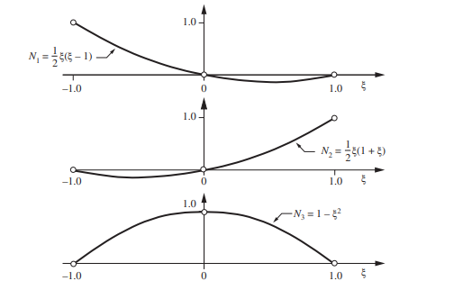
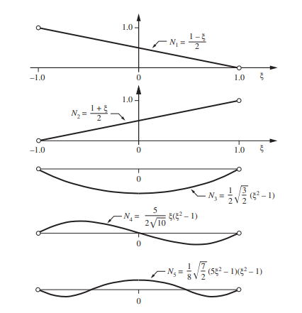
The standard polynomial basis functions, called shape functions, can be defined in various ways. We will consider shape functions based on Lagrange polynomials and Legendre ${ }^{12}$ polynomials. We will use the same notation for both types of shape function.
Lagrange shape functions
Lagrange shape functions of degree $p$ are constructed by partitioning $I_{\mathrm{st}}$ into $p$ sub-intervals. The length of the sub-intervals is typically $2 / p$ but the lengths may vary. The node points are $\xi_{1}=-1$, $\xi_{2}=1$ and $-1<\xi_{3}<\xi_{4}<\cdots<\xi_{p+1}<1$. The $i$ th shape function is unity in the $i$ th node point and is zero in the other node points:
$$
N_{i}(\xi)=\prod_{\substack{k=1 \ k \neq i}}^{p+1} \frac{\xi-\xi_{k}}{\xi_{i}-\xi_{k}}, \quad i=1,2, \ldots, p+1, \quad \xi \in I_{\mathrm{st}}
$$
These shape functions have the following important properties:
$$
N_{i}\left(\xi_{j}\right)=\left{\begin{array}{ll}
1 & \text { if } i=j \
0 & \text { if } i \neq j
\end{array} \quad \text { and } \sum_{i=1}^{p+1} N_{i}(\xi)=1 .\right.
$$
For example, for $p=2$ the equally spaced node points are $\xi_{1}=-1, \xi_{2}=1, \xi_{3}=0$. The corresponding Lagrange shape functions are illustrated in Fig. 1.3.
数学代写|计算方法代写computational method代考|Finite element spaces in one dimension
We are now in a position to provide a precise definition of finite element spaces in one dimension.
The domain $I={x \mid 0<x<\ell}$ is partitioned into $M$ non-overlapping intervals called finite elements. A partition, called finite element mesh, is denoted by $\Delta$. Thus $M=M(\Delta)$. The boundary points of the elements are the node points. The coordinates of the node points, sorted in ascending order, are denoted by $x_{i},(i=1,2, \ldots, M+1)$ where $x_{1}=0$ and $x_{M+1}=\ell$. The $k$ th element $I_{k}$ has the boundary points $x_{k}$ and $x_{k+1}$, that is, $I_{k}=\left{x \mid x_{k}<x<x_{k+1}\right}$.
Various approaches are used for the construction of sequences of finite element mesh. We will consider four types of mesh design:
- A mesh is uniform if all elements have the same size. On the interval $I=(0, \ell)$ the node points are located as follows:
$$
x_{k}=(k-1) \ell / M(\Delta) \text { for } k=1,2,3, \ldots, M(\Delta)+1 .
$$ - A sequence of meshes $\Delta_{K}(K=1,2, \ldots)$ is quasiuniform if there exist positive constants $C_{1}, C_{2}$, independent of $K$, such that
$$
C_{1} \leq \frac{\ell_{\max }^{(K)}}{\ell_{\min }^{(K)}} \leq C_{2}, \quad K=1,2, \ldots
$$
where $\ell_{\max }^{(K)}$ (resp. $\ell_{\min }^{(K)}$ ) is the length of the largest (resp. smallest) element in mesh $\Delta_{K}$. In two and three dimensions $\ell_{k}$ is defined as the diameter of the $k$ th element, meaning the diameter of the smallest circle or sphere that envelopes the element. For example, a sequence of quasiuniform meshes would be generated in one dimension if, starting from an arbitrary mesh, the elements would be successively halved. - A mesh is geometrically graded toward the point $x=0$ on the interval $0<x<\ell$ if the node points are located as follows:
$$
x_{k}= \begin{cases}0 & \text { for } k=1 \ q^{M(\Delta)+1-k} \ell & \text { for } k=2,3, \ldots, M(\Delta)+1\end{cases}
$$
where $0<q<1$ is called grading factor or common factor. These are called geometric meshes. - A mesh is a radical mesh if on the interval $01, \quad k=1,2, \ldots, M(\Delta)+1 .
$$
The question of which of these schemes is to be preferred in a particular application can be answered on the basis of a priori information concerning the regularity of the exact solution and aspects of implementation. Practical considerations that should guide the choice of the finite element mesh will be discussed in Section 1.5.2.
计算方法代写
数学代写|计算方法代写computational method代考|Approximate solutions
上一节中定义的试验空间和测试空间是无限维的,即它们跨越无限多个线性独立函数。为了找到一个近似解,我们构造了有限维子空间,分别表示为小号⊂X,在⊂是并寻求功能在∈小号满足乙(在,在)=F(在)对全部在∈在. 让我们回到章节中描述的介绍性示例1.1并定义
在=在n=∑j=1n一种j披j,在=在n=∑一世=1nb一世披一世
在哪里披一世(一世=1,2,…n)是基函数。使用定义ķ一世j和米一世j在等式中给出。(1.12),我们将双线性形式写为
乙(在,在)≡∫0吨(ķ在′在′+C在在)dX=∑一世=1n∑j=1n(ķ一世j+米一世j)一种jb一世 =b吨([ķ]+[米])一种
相似地,
F(在)≡∫0ℓF在dX=∑一世=1nb一世r一世=b吨r
在哪里r一世在等式中定义。(1.12)。因此我们可以写乙(在,在)−F(在)=0采用以下形式:
b吨(([ķ]+[米])一种−r)=0.
由于这必须适用于任何选择b, 它遵循
([ķ]+[米])一种=r
这与我们在最小化积分 I 时需要求解的线性方程组相同,参见方程。(1.14)。当然,这不是巧合。广义问题的解决方案:“找到在n∈小号这样乙(在n,在)=F(在)对全部在∈在n,最小化能量范数的误差。见定理 1.4。
定理1.3错误和被定义为和=在−在n满足乙(和,在)=0对全部在∈小号0(一世). 这个结果直接来自
乙(在,在)=F(在) 对全部 在∈小号0(一世) 乙(在n,在)=F(在) 对全部 在∈小号0(一世).
从我们得到的第一个方程中减去第二个方程,
乙(在−在n,在)≡乙(和,在)=0 对全部 在∈小号0(一世).
这个方程被称为 Galerkin11正交性条件。
定理 1.4 如果在n∈小号0(一世)满足乙(在n,在)=F(在)对全部在∈小号0(一世)然后在n最小化错误在和X−在n在能量规范中在和X是确切的解决方案:
|在和X−在n|和(一世)=分钟在∈小号¯|在和X−在|和(一世).
证明:让和=在−在n然后让在是一个任意函数小号0(一世). 然后
|和+在|和(l)2≡12乙(和+在,和+在)=12乙(和,和)+乙(和,在)+12乙(在,在).
右边的第一项是|和|和(一世)2, 由于定理,第二项为零1.3,第三项对任何一个都是正的在≠0在小号∘(一世). 所以|和|和(一世)是最小值。
定理1.4指出错误取决于问题的确切解决方案在和X以及试验空间的定义小号¯(一世).
有限元法是构建试验空间的一种灵活而强大的方法。以下部分概述了有限元方法的基本算法结构。
数学代写|计算方法代写computational method代考|The standard polynomial space
标准多项式空间p,表示为小号p(一世英石 ), 由单项式跨越1,X,X2,…,Xp在标准元素上定义
一世英石 =X∣−1<X<1.
基函数的选择取决于实现的考虑、保持系数矩阵的条件数较小以及个人偏好。对于这里考虑的对称正定矩阵,条件数C是最大特征值除以最小值。解决线性问题时丢失的位数大致等于日志10C. 在此上下文中应理解将条件数表征为大或小。在有限元法中,条件数取决于基函数和网格的选择。
标准多项式基函数,称为形状函数,可以用多种方式定义。我们将考虑基于拉格朗日多项式和勒让德的形状函数12多项式。我们将对两种类型的形状函数使用相同的符号。
拉格朗日形函数
度数的拉格朗日形函数p是通过分区构造的一世s吨进入p子区间。子区间的长度通常为2/p但长度可能会有所不同。节点点是X1=−1, X2=1和−1<X3<X4<⋯<Xp+1<1. 这一世形状函数是统一的一世th 节点点并且在其他节点点中为零:
ñ一世(X)=∏ķ=1 ķ≠一世p+1X−XķX一世−Xķ,一世=1,2,…,p+1,X∈一世s吨
这些形状函数具有以下重要性质:
$$
N_{i}\left(\xi_{j}\right)=\left{1 如果 一世=j 0 如果 一世≠j\quad \text { 和 } \sum_{i=1}^{p+1} N_{i}(\xi)=1 .\right.
$$
例如,对于p=2等间距的节点点是X1=−1,X2=1,X3=0. 相应的拉格朗日形函数如图 1.3 所示。
数学代写|计算方法代写computational method代考|Finite element spaces in one dimension
我们现在可以提供一维有限元空间的精确定义。
域名一世=X∣0<X<ℓ被划分为米非重叠区间称为有限元。称为有限元网格的分区表示为Δ. 因此米=米(Δ). 元素的边界点是节点。节点点的坐标,按升序排列,表示为X一世,(一世=1,2,…,米+1)在哪里X1=0和X米+1=ℓ. 这ķ元素一世ķ有边界点Xķ和Xķ+1, 那是,I_{k}=\left{x \mid x_{k}<x<x_{k+1}\right}I_{k}=\left{x \mid x_{k}<x<x_{k+1}\right}.
各种方法用于构建有限元网格序列。我们将考虑四种类型的网格设计:
- 如果所有元素的大小相同,则网格是均匀的。在区间一世=(0,ℓ)节点位置如下:
Xķ=(ķ−1)ℓ/米(Δ) 为了 ķ=1,2,3,…,米(Δ)+1. - 一系列网格Δķ(ķ=1,2,…)如果存在正常数是准均匀的C1,C2, 独立于ķ, 这样
C1≤ℓ最大限度(ķ)ℓ分钟(ķ)≤C2,ķ=1,2,…
在哪里ℓ最大限度(ķ)(分别。ℓ分钟(ķ)) 是网格中最大(或最小)元素的长度Δķ. 在二维和三维ℓķ被定义为直径ķth 元素,表示包围该元素的最小圆或球体的直径。例如,如果从任意网格开始,元素将连续减半,则将在一维中生成一系列准均匀网格。 - 网格朝向该点进行几何分级X=0在区间0<X<ℓ如果节点点的位置如下:
Xķ={0 为了 ķ=1 q米(Δ)+1−ķℓ 为了 ķ=2,3,…,米(Δ)+1
在哪里0<q<1称为分级因子或公因子。这些被称为几何网格。 - 一个网格是一个激进的网格,如果在区间上01,ķ=1,2,…,米(Δ)+1.可以根据有关确切解决方案的规律性
和实施方面的先验信息来回答在特定应用中优先选择这些方案中的哪一个的问题。指导有限元网格选择的实际考虑将在 1.5.2 节中讨论。

统计代写请认准statistics-lab™. statistics-lab™为您的留学生涯保驾护航。
金融工程代写
金融工程是使用数学技术来解决金融问题。金融工程使用计算机科学、统计学、经济学和应用数学领域的工具和知识来解决当前的金融问题,以及设计新的和创新的金融产品。
非参数统计代写
非参数统计指的是一种统计方法,其中不假设数据来自于由少数参数决定的规定模型;这种模型的例子包括正态分布模型和线性回归模型。
广义线性模型代考
广义线性模型(GLM)归属统计学领域,是一种应用灵活的线性回归模型。该模型允许因变量的偏差分布有除了正态分布之外的其它分布。
术语 广义线性模型(GLM)通常是指给定连续和/或分类预测因素的连续响应变量的常规线性回归模型。它包括多元线性回归,以及方差分析和方差分析(仅含固定效应)。
有限元方法代写
有限元方法(FEM)是一种流行的方法,用于数值解决工程和数学建模中出现的微分方程。典型的问题领域包括结构分析、传热、流体流动、质量运输和电磁势等传统领域。
有限元是一种通用的数值方法,用于解决两个或三个空间变量的偏微分方程(即一些边界值问题)。为了解决一个问题,有限元将一个大系统细分为更小、更简单的部分,称为有限元。这是通过在空间维度上的特定空间离散化来实现的,它是通过构建对象的网格来实现的:用于求解的数值域,它有有限数量的点。边界值问题的有限元方法表述最终导致一个代数方程组。该方法在域上对未知函数进行逼近。[1] 然后将模拟这些有限元的简单方程组合成一个更大的方程系统,以模拟整个问题。然后,有限元通过变化微积分使相关的误差函数最小化来逼近一个解决方案。
tatistics-lab作为专业的留学生服务机构,多年来已为美国、英国、加拿大、澳洲等留学热门地的学生提供专业的学术服务,包括但不限于Essay代写,Assignment代写,Dissertation代写,Report代写,小组作业代写,Proposal代写,Paper代写,Presentation代写,计算机作业代写,论文修改和润色,网课代做,exam代考等等。写作范围涵盖高中,本科,研究生等海外留学全阶段,辐射金融,经济学,会计学,审计学,管理学等全球99%专业科目。写作团队既有专业英语母语作者,也有海外名校硕博留学生,每位写作老师都拥有过硬的语言能力,专业的学科背景和学术写作经验。我们承诺100%原创,100%专业,100%准时,100%满意。
随机分析代写
随机微积分是数学的一个分支,对随机过程进行操作。它允许为随机过程的积分定义一个关于随机过程的一致的积分理论。这个领域是由日本数学家伊藤清在第二次世界大战期间创建并开始的。
时间序列分析代写
随机过程,是依赖于参数的一组随机变量的全体,参数通常是时间。 随机变量是随机现象的数量表现,其时间序列是一组按照时间发生先后顺序进行排列的数据点序列。通常一组时间序列的时间间隔为一恒定值(如1秒,5分钟,12小时,7天,1年),因此时间序列可以作为离散时间数据进行分析处理。研究时间序列数据的意义在于现实中,往往需要研究某个事物其随时间发展变化的规律。这就需要通过研究该事物过去发展的历史记录,以得到其自身发展的规律。
回归分析代写
多元回归分析渐进(Multiple Regression Analysis Asymptotics)属于计量经济学领域,主要是一种数学上的统计分析方法,可以分析复杂情况下各影响因素的数学关系,在自然科学、社会和经济学等多个领域内应用广泛。
MATLAB代写
MATLAB 是一种用于技术计算的高性能语言。它将计算、可视化和编程集成在一个易于使用的环境中,其中问题和解决方案以熟悉的数学符号表示。典型用途包括:数学和计算算法开发建模、仿真和原型制作数据分析、探索和可视化科学和工程图形应用程序开发,包括图形用户界面构建MATLAB 是一个交互式系统,其基本数据元素是一个不需要维度的数组。这使您可以解决许多技术计算问题,尤其是那些具有矩阵和向量公式的问题,而只需用 C 或 Fortran 等标量非交互式语言编写程序所需的时间的一小部分。MATLAB 名称代表矩阵实验室。MATLAB 最初的编写目的是提供对由 LINPACK 和 EISPACK 项目开发的矩阵软件的轻松访问,这两个项目共同代表了矩阵计算软件的最新技术。MATLAB 经过多年的发展,得到了许多用户的投入。在大学环境中,它是数学、工程和科学入门和高级课程的标准教学工具。在工业领域,MATLAB 是高效研究、开发和分析的首选工具。MATLAB 具有一系列称为工具箱的特定于应用程序的解决方案。对于大多数 MATLAB 用户来说非常重要,工具箱允许您学习和应用专业技术。工具箱是 MATLAB 函数(M 文件)的综合集合,可扩展 MATLAB 环境以解决特定类别的问题。可用工具箱的领域包括信号处理、控制系统、神经网络、模糊逻辑、小波、仿真等。