统计代写|金融统计代写Financial Statistics代考|Probability of Union
To assess the probability of union, first, imagine we randomly select one card from the deck. Let event $A={$ club $}$ and event $B={$ heart or diamond $}$. Let $A \cup B$ denote the union, so $A \cup B={$ club, heart, diamond $}$.
The union of $A$ and $B$ means the event ” $A$ or $B$ ” occurs. We can now compute the mathematical probability of $A$ or $B$ : $$ P(A)=\frac{13}{52}=\frac{1}{4} \text { and } P(B)=\frac{13+13}{52}=\frac{1}{2} $$
The probability of getting a club, a heart, or a diamond is obtained by adding the number of club, heart, and diamond cards and dividing by the total number of cards, 52. As a result, the probability of drawing a card that is a member of the union of these two events is $$ P(A \cup B)=P(A)+P(B)=\frac{1}{4}+\frac{1}{2}=\frac{3}{4} $$ Thus, we have a $\frac{3}{4}=75 \%$ chance of randomly drawing a single card that is a club or a heart or a diamond.
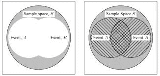
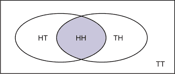
If $A$ and $B$ are mutually exclusive, the probability formula for a union of $A$ and $B$ is $$ P(A \cup B)=P(A)+P(B) $$ The rule for obtaining the probability of the union of $A$ and $B$ as indicated in Eq. $5.4$ is the addition rule for two events that are mutually exclusive. This addition rule is illustrated by the Venn diagram in Fig. 5.9, where we note that the area of two circles taken together (denoting $A \cup B$ ) is the sum of the areas of the two circles.
统计代写|金融统计代写Financial Statistics代考|Probability of Intersection
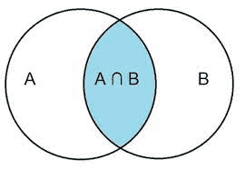
If $A={$ diamond $}$ and $B={$ diamond or heart $}$, then $A \cap B={$ diamond $}=$ set of points that are in both $A$ and $B$. Using Table 5.2, we obtain $$ \begin{aligned} P(A) & =\frac{13}{52}=\frac{1}{4} \ P(B) & =(13+13) / 52=\frac{1}{2} \ P(A \cap B) & =\frac{13}{52}=\frac{1}{4} \end{aligned} $$ Thus, the probability of drawing a diamond and drawing a diamond or a heart is the probability of drawing a diamond, which is $\frac{1}{4}$, or $25 \%$. From Eq. 5.5, we can define the probability of an intersection as $$ P(A \cap B)=P(A)+P(B)-P(A \cup B) $$ If, instead, $A=$ all diamonds and $B=$ all diamonds or all hearts, then $$ P(A \cap B)=\frac{1}{4}+\frac{1}{2}-\frac{1}{2}=\frac{1}{4} $$
统计代写|金融统计代写Financial Statistics代考|Probabilities of Outcomes
The probability of an event is ā real number on a scale from 0 to 1 thât measures the likelihood of the event’s occurring. If an outcome (or event) has a probability of 0 , then its occurrence is impossible; if an outcome (or event) has a probability of 1.0, then its occurrence is certain. Getting either a head or a tail in a coin toss is an example of an event that has a probability of $1.0$. Because there are only two possibilities, either one event or the other is certain to occur. An event with a zero probability is an impossible event, such as getting both a head and a tail when tossing a coin once.
When we roll a fair die, we are just as likely to obtain any face of the die as any other. Because there are six faces to a die, we generally say the “outcome” of the toss can be one of six numbers: $1,2,3,4,5,6$.
The probability of an outcome can be calculated by the classical approach, the relative frequency approach, or the subjective approach. The first two approaches are discussed in this section, the third approach in the next.
Classical probability is often called a priori probability, because if we keep using orderly examples, such as fair coins and unbiased dice, we can state the answer in advance (a priori) without tossing a coin or rolling a die. In other words, we can make statements based on logical reasoning before any experiments take place. Classical probability defines the probability that an event will occur as $$ \text { Probability of an event }=\frac{\text { number of outcomes containéd in the event }}{\text { total number of possible outcomes }} $$ Note that this approach is applicable only when all basic outcomes in the sample space are equally probable. For example, the probability of getting a tail upon tossing a fair coin is $$ P(\text { tail })=\frac{1}{1+1}=\frac{1}{2} $$
And for the die-rolling example, the probability of obtaining the face 4 is $$ P(4)=\frac{1}{6} $$ The relative frequency approach to calculating probability requires the random experiment to take place as defined in Eq. 5.2: $$ P\left(o=e_i\right)=\frac{n_i}{N} \quad \text { or } \quad P\left(e_i\right)=\frac{n_i}{N} $$
统计代写|金融统计代写Financial Statistics代考|Subjective Probability
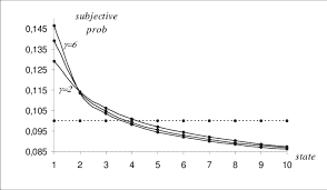
An alternative view about probability, which does not depend on the concept of repeatable random experiments, defines probability in terms of a subjective, or personalistic, concept. According to this concept of subjective probability, the probability of an event is the degree of belief, or degree of confidence, an individual places in the occurrence of an event on the basis of whatever evidence is available. This evidence may be data on the relative frequency of past occurrences, or it may be just an educated guess. The individual may assign an event the probability of 1 , 0 , or any other number between those two. Here are a few examples of situations that require a subjective probability:
An individual consumer assigns a probability to the event of purchasing a TV during the next quarter.
A quality control manager asserts the probability that a future incoming shipment will have $1.5 \%$ or fewer defective items.
An auditing firm wishes to determine the probability that an audited voucher will contain an error.
An investor ponders the probability that the Dow Jones closing index will be below 3,000 at some time during a 3-month period beginning on November 10, 1992.
As we have stated, an event is the result of a random experiment consisting of one or more basic outcomes. If an event consists of only one basic outcome, it is a simple event; if it consists of more than one basic outcome, it is a composite event. In the die-rolling experiment discussed in Fig. 5.1, the sample space is $S={1,2,3$, $4,5,6}$
Suppose we are interested in the event $E$, where the outcome is 1 or 6 . We can clearly describe the event $E$ as $E={1.6}$. An event $E$ is a subset of the sample space $S$. This is a composite event because it includes the simple events ${1}$ and ${6}$. The subset definition enables us to define an event in general.
In the tossing of a fair die, suppose that event $A$ represents the faces $1,2,3,4$, and 5 and event $B$ the faces of 4,5 , and 6 . Graphically, the relationship between basic outcomes and events can be represented as shown in Fig. 5.6. The intersection of these two events is the faces 4 and 5 , because these faces are common to both events.
统计代写|金融统计代写Financial Statistics代考|Random Experiment, Outcomes, Sample Space
A random experiment is a process that has at least two possible outcomes and is characterized by uncertainty as to which will occur. Each of the following examples involves a random experiment:
A die is rolled.
A voter is asked which of four candidates he or she prefers.
A person is asked whether President Bush should order US troops to liberate Kuwait.
The daily change in the price of silver per ounce is observed. When a die is rolled, the set of basic outcomes comprises 1 through 6; these basic outcomes represent the various possibilities that can occur. In other words, the possible outcomes of a random experiment are called the basic outcomes. The set of all basic outcomes is called the sample space. Thus, basic outcomes are equivalent to sample points in a sample space.
Suppose you are interested in getting an even number in rolling a die; in this case, the event is rolling a 2,4 , or 6 , which is a subset of ${1,2,3.4,5,6}$. In other words, an event is a set of basic outcomes from the sample space, and it is said to occur if the random experiment gives rise to one of its constituent basic outcomes. Each basic outcome within each event (e.g., ${2}{4}{6}$ ) can also be called a simple event. Hence, an event is a collection of one or more simple events. Finally, a basic event is a subset of the sample space. The concepts of random experiment, outcomes, sample space, and event, then, are fundamental to an understanding of probability.
The starting point of probability is the random experiment. Random experiments have three properties:
They can be repeated physically or conceptually.
The set consisting of all of possible outcomes – that is, the sample space-can be specified in advance.
Various repetitions do not always yield the same outcome. Simple examples of conducting a random experiment include rolling dice, tossing a coin, and drawing a card from a deck of 52 playing cards.
Because of uncertainty in the business environment, business decision making is a tricky and an important skill. If the executive knew the exact outcomes of the courses of action available, he or she would have no difficulty making optimal decisions. However, the executive generally does not know the exact outcome of a decision. Thus, business executives spend much time evaluating the probabilities of various alternative outcomes. For example, an executive may need to determine the probability of extensive employee turnover if the firm moves to another area. Or a business decision maker may want to evaluate the impact of changes in economic indicators such as interest rate, inflation, and gross national product (GNP) on a company’s future earnings.
统计代写|金融统计代写Financial Statistics代考|Sample Space of an Experiment and the Venn Diagram
For convenience, we can represent each outcome of a random experiment by a set of symbols. The symbol $S$ is used to represent the sample space of the experiment. As we have noted, the sample space is the set of all basic outcomes (simple events) of the random experiment. In the foregoing die-rolling example, the sample space is $S={1,2,3,4,5,6}$. When a person takes a driver’s license test, the sample space contains only two elements: $S={P, F}$, where $P$ indicates a pass and $F$ a failure. In a stock price forecast, the sample space could contain three elements: $S={U, D$, $N}$, where $U, D$, and $N$ represent movement up, movement down, and no change in the price of a stock. In sum, the different basic outcomes of an experiment are often referred to as sample points (simple events), and the set of all possible outcomes is called the sample space. Thus, the sample points (simple events) form the sample space.
A Venn diagram can be used to describe graphically various basic outcomes (simple events) in a sample space. The rectangle represents the sample space, and the points are basic outcomes. Events are usually represented by circles or rectangles. Figure $5.1$ shows a Venn diagram. The elements labeled represent the six basic outcomes of rolling a die. In Fig. 5.2, the circle indicates the event of all even numbers that can result from rolling a single die. Let event $A={2,4,6}$. Again, the sample space is the possible outcomes of rolling a die. Figure $5.3$ shows events $A={1,3}$ and $B={4,5}$. When two events have no basic outcome in common, they are said to be mutually exclusive events. When events have some elements in common, the intersection of the events is the event that consists of the common elements. Say we have one event $A={2,3,4,6}$ and another event $B={2,3,5}$. The intersection of these events is shown in Fig. 5.4. The common elements are 2 and 3 .
All data tables have four elements: a caption, column labels, row labels, and cells. The caption describes the information that is contained in the table. The column labels identify the information in the columns, such as the gross national product, the inflation rate, or the Dow Jones Industrial Average. Examples of row labels include years, dates, and states. A cell is defined by the intersection of a specific row and a specific column.
Example 2.2 Annual CPI, T-Bill Rate, and Prime Rate. To illustrate, Table $2.1$ gives some macroeconomic information from 1950 to 2010 . The caption is “CPI, T-bill rate, and prime rate (1950-2010).” The row labels are the years 1950-2010. The column labels are CPI (consumer pace index), 3-month T-bill rate, and prime rate. Changes in the consumer price index, the most commonly used indicator of the economy’s price level, are a measure of inflation or deflation. (For a more detailed description of the CPI, see Chap. 19.) The 3-month T-bill interest rate is the interest rate that the USA Treasury pays on 91-day debt instruments, and the prime rate is the interest rate that banks charge on loans to their best customers, usually large firms. This table, then, presents macroeconomic information for any year indicated. For example, the CPI for 2010 was $218.1$ and the prime rate in 2008 was $5.09 \%$. The relationship between the CPI and 3-month T-bill rate will be discussed in Chap. $19 .$
统计代写|金融统计代写Financial Statistics代考|Data Presentation: Charts and Graphs
It is sometimes said that a picture is worth a thousand words, and nowhere is this statement more true than in the analysis of data. Tables are usually filled with highly specific data that take time to digest. Graphs and charts, though they are often less detailed than tables, have the advantage of presenting data in a more accessible and memorable form. In most graphs and charts, the independent variable is plotted on the horizontal axis (the $x$-axis) and the dependent variable on the vertical axis (the $y$-axis). Frequently, “time” is plotted along the $x$-axis. Such a graph is known as a time-series graph because on it, changes in a dependent variable (such as GDP, inflation rate, or stock prices) can be traced over time.
Line charts are constructed by graphing data points and drawing lines to connect the points. Figure $2.1$ shows how the rate of return on the S\&P 500 and the 3-month T-bill rate have varied over time. ${ }^1$ The independent variable is the year (ranging from 1990 to 2010), so this is a time-series graph. The dependent variables are often in percentages.
Figure $2.2$ is a graph of the components of the gross domestic product (GDP)personal consumption, government expenditures, private investment, and net exports-over time. This is also a time-series graph because the independent variable is time. It is a component-parts line chart. These series have been “deflated” by expressing dollar amounts in constant 2005 dollars. (Chap. 19 discusses the deflated series in further detail.)
Figure $2.2$ is also called a component-parts line graph because the four parts of the GDP are graphed. The sum of the four components equals the GDP. Using this type of graph makes it possible to show the sources of increases or declines in the GDP. (The data used to generate Fig. $2.2$ are found in Table 2.2.)
Bar charts can be used to summarize small amounts of information. Figure $2.3$ shows the average annual returns for Tri-Continental Corporation for investment periods of seven different durations ending on September 30, 1991. This figure shows that Tri-Continental has provided investors double-digit returns during a 50-year period.
It also shows that the investment performance of this company was better than that of the Dow Jones Industrial Average (DJIA) and the S\&P $500 .^2$
统计代写|金融统计代写Financial Statistics代考|Deductive Versus Inductive Analysis in Statistics
We also encounter another dichotomy in statistical analysis. Deduction is the use of general information to draw conclusions about specific cases. For example, probability tells us that if a student is chosen by lottery from a calculus class composed of 60 mathematics majors and 40 business administration majors, then the odds against picking a mathematics majors are 4-6. Thus we can deduce that about $40 \%$ of such single-member samples of the students in this calculus class will be business administration majors. As another example of deduction, consider a firm that learns that $1 \%$ of its auto parts are defective and concludes that in any random sample, $1 \%$ of its parts are therefore going to be defective. The use of probability to determine the chance of obtaining a particular kind of sample result is known as deductive statistical analysis. In Chaps. 5, 6, and 7, we will learn how to apply deductive techniques when we know everything about the population in advance and are concerned with studying the characteristics of the possible samples that may arise from that known population. Induction involves drawing general conclusions from specific information. In statistics, this means that on the strength of a specific sample, we infer something about a general population. The sample is all that is known; we must determine the uncertain characteristics of the population from the incomplete information available. This kind of statistical analysis is called inductive statistical analysis. For example, if $56 \%$ of a sample prefers a particular candidate for a political office, then we can estimate that $56 \%$ of the population prefers this candidate. Of course, our estimate is subject to error, and statistics enables us to calculate the possible error of an estimate. In this example, if the error is $3 \%$ points, it can be inferred that the actual percentage of voters preferring the candidate is $56 \%$ plus or minus $3 \%$; that is, it is between $53 \%$ and $59 \%$.
Deductive statistical analysis shows how samples are generated from a population, and inductive statistical analysis shows how samples can be used to infer the characteristics of a population. Inductive and deductive statistical analyses are fully complementary. We must study how samples are generated before we can learn to generalize from a sample.
统计代写|金融统计代写Financial Statistics代考|Data Collection
After identifying a research problem and selecting the appropriate statistical methodology, researchers must collect the data that they will then go on to analyze. There are two sources of data: primary and secondary sources. Primary data are data collected specifically for the study in question. Primary data may be collected by methods such as personal investigation or mail questionnaires. In contrast, secondary data were not originally collected for the specific purpose of the study at hand but rather for some other purpose. Examples of secondary sources used in finance and accounting include the Wall Street Journal, Barron’s, Value Line Investment Survey, Financial Times, and company annual reports. Secondary sources used in marketing include sales reports and other publications. Although the data provided in these publications can be used in statistical analysis, they were not specifically collected for that use in any particular study.
Example 2.1 Primary and Secondary Sources of Data. Let us consider the following cases and then characterize each data source as primary or secondary:
(Finance) To determine whether airline deregulation has increased the return and risk of stocks issued by firms in the industry, a researcher collects stock data from the Wall Street Journal and the Compustat database. (The Compustat database contains accounting and financial information for many firms.)
(Production) To determine whether ball bearings meet measurement specifications, a production engineer examines a sample of 100 bearings.
(Marketing) Before introducing a hamburger made with a new recipe, a firm gives 25 customers the new hamburger and asks them on a questionnaire to rate the hamburger in various categories.
(Political science) A candidate for political office has staff members call 1,000 voters to determine what candidate they prefer in an upcoming election.
(Marketing) A marketing firm looks up, in Consumer Reports, the demand for different types of cars in the United States.
统计代写|金融统计代写Financial Statistics代考|The Role of Statistics in Business and Economics
Statistics is a body of knowledge that is useful for collecting, organizing, presenting, analyzing, and interpreting data (collections of any number of related observations) and numerical facts. Applied statistical analysis helps business managers and economic planners formulate management policy and make business decisions more effectively. And statistics is an important tool for students of business and economics. Indeed, business and economic statistics has become one of the most important courses in business education, because a background in applied statistics is a key ingredient in understanding accounting, economics, finance, marketing, production, organizational behavior, and other business courses.
We may not realize it, but we deal with and interpret statistics every day. For example, the Dow Jones Industrial Average (DJIA) is the best-known and most widely watched indicator of the direction in which stock market values are heading. When people say, “The market was up 12 points today,” they are probably referring to the DJIA. This single statistic summarizes stock prices of 30 large companies. Rather than listing the prices at which all of the approximately 2,000 stocks traded on the New York Stock Exchange are currently selling, analysts and reporters often cite this one number as a measure of overall market performance.
Let’s take another example. Before elections, the media sometimes present surveys of voter preference in which a sample of voters instead of the whole population of voters is asked about candidate preferences. The media usually give the results of the poll and then state the possible margin of error. A margin of error of $3 \%$ means that the actual extent of a candidate’s popular support may differ from the poll results by as much as $3 \%$ points in either direction (“plus or minus”). Anyone who conducts a survey must understand statistics in order to make such decisions as how many people to contact, how to word the survey, and how to calculate the potential margin of error.
In business and industry, managers frequently use statistics to help them make better decisions. A shoe manufacturer, for instance, needs to produce a forecast of future sales in order to decide whether to expand production. Sales forecasts provide statistical guidance in most business decision making.
On a broader scale, the government publishes a variety of data on the health of the economy. Some of the most popular measures are the gross national product (GNP), the index of leading economic indicators, the unemployment rate, the money supply, and the consumer price index (CPI). All these measures are statistics that are used to summarize the general state of the economy. And, of course, business, government, and academic economists use statistical methods to try to predict these macroeconomic and other variables.
The following additional examples are presented to show that the use of statistics is widespread not only in business and economics but in everyday life as well.
统计代写|金融统计代写Financial Statistics代考|Descriptive Versus Inferential Statistics
Having gotten a feel for the use of statistics by looking at several illustrations, we can now refine our definition of the term. Statistics is the collection, presentation, and summary of numerical information in such a way that the data can be easily interpreted.
There are two basic types of statistics: descriptive and inferential. Descriptive statistics deals with the presentation and organization of data. Measures of central tendency, such as the mean and median, and measures of dispersion, such as the standard deviation and range, are descriptive statistics. These types of statistics summarize numerical information. For example, a teacher who calculates the mean, median, range, and standard deviation of a set of exam scores is using descriptive statistics. Descriptive statistics is the subject of the first part of this book. The following are examples of the use (or misuse) of descriptive statistics. Example 1.6 Baseball Players’ Batting Averages. Descriptive statistics can be used to provide a point of reference. The batting averages of baseball players are commonly reported in the newspapers, but to people unfamiliar with baseball, these numbers may be misleading. For example, Wade Boggs of the Boston Red Sox hit $.366$ in 1988; that is, he got a hit in almost $37 \%$ of his official at bats. Because he was unsuccessful over $63 \%$ of the time, however, a person with little knowledge of baseball might conclude that Boggs is an inferior hitter. Comparing Boggs’s average to the mean batting average of all players in the same year, which was $.285$, reveals that Boggs is among the best hitters.
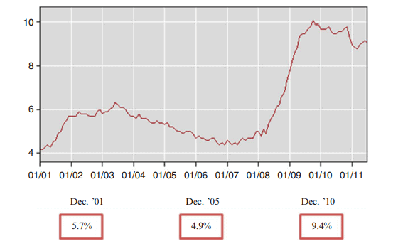
Example 1. 7 Monthly Unemployment Rates. Graphical statistical analysis can be used to summarize small amounts of information. Figure $1.1$ displays the US unemployment rates for each month from January 2001 to July 2011. It shows, for instance, that the unemployment rates for December 2001, December 2005, and December 2010 were $5.7 \%, 4.9 \%$, and $9.4 \%$, respectively.
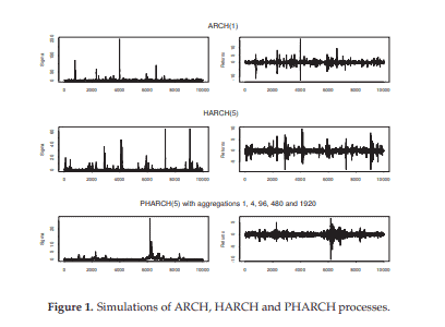
统计代写|金融统计代写Financial Statistics代考|High Frequency Data
In this section we further elaborate on high frequency data and introduce the series that will be analyzed later. High frequency data are very important in the financial environment, mainly because there exist large movements in short intervals of time. This aspect represents an interesting opportunity for trading. Furthermore, it is well known that volatilities in different frequencies have significant cross-correlation. We can even say that coarse volatility predicts fine volatility better than the inverse, as shown in Dacorogna et al. (2001).
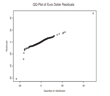
As an example, take the tick by tick foreign exchange (FX) time series Euro-Dollar, from January First 1999 to December 31, 2002. Returns are calculated using bid and ask prices, as $$ r_{t}=\ln \left(\left(p_{t}^{b i d}+p_{t}^{a s k}\right) / 2\right)-\ln \left(\left(p_{t-1}^{b i d}+p_{t-1}^{a s k}\right) / 2\right) $$ We discard Saturdays and Sundays, and we replace holidays with the means of the last ten observations of the returns for each respective hour and day. After cleaning the data (see Dacorogna et al. (2001), for details) we will consider equally spaced returns, with sampling interval $\Delta t=15 \mathrm{~min}$. This seems to be adequate, as many studies indicate.
Figure 2 shows Euro-Dollar returns calculated as above. The length of this time series is 95,317 . The figure shows that the absolute returns present a seasonal pattern. This is due to the fact that physical time does not follow, necessarily, the same pattern as the business time. This is a typical behavior of a financial time series and we will use a seasonal adjustment procedure similar to that of Martens et al. (2002). However, we will use absolute returns instead of squared returns; that is, we will compute the seasunal patturn as $$ S_{d_{,}, h}=\frac{1}{s} \sum_{j=1}^{s} \mid\left(r_{d_{t}, j, t} \mid,\right. $$ where $r_{d, s, t}$ is the return in the weekday $d$, week $s$ and hour $h$, and $s$ is the number of weeks from the beginning of the series. Therefore, $S_{d, N}, N_{t}$ is the rolling window mean of the absolute returns with the beginning fixed.
In Figure 3 we have the autocorrelation function of these returns and of squared returns. The seasonality pattern is no longer present.
FX data has some distinct characteristics, mainly because they are produced twenty four hours a day, seven days a week. In particular, Euro-Dollar is the most liquid FX in the world. However, there are periods where the activity is greater or smaller, causing seasonal patterns to occur, as seen above. Let us analyze some facts about these returns that we will denote simply by rt. We can see in Figure 4 the histogram fitted with a non-parametric density kernel estimate, using unbiased cross-validation method to estimate the bandwidth. It shows fat tails and high kurtosis, namely, 121 , while its skewness coefficient is $-0.079$, showing almost symmetry. A normality test (Jarque-Bera) rejects the hypothesis that these returns are normal.
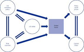
统计代写|金融统计代写Financial Statistics代考|Introduction and Motivation
A financial asset is referred to as a “safe haven” asset if it provides hedging benefits during periods of market turbulence. In other words, during periods of market stress, “safe haven” assets are supposed to be uncorrelated, or negatively correlated, with large markets slumps experienced by more traditional financial assets (typically stock or bond prices).
The financial literature identifies various asset classes exhibiting “safe haven” features: gold and other precious metals, the exchange rates of some key international currencies against the US dollar, oil and other important agricultural commodities, and US long-term government bonds.
This paper contributes to the existing literature focusing on some of the most representative “safe haven” assets, namely gold, the Swiss Franc/US dollar exchange rate, and oil. The main motivation behind this choice is twofold.
First, empirical research on these assets have attracted major attention in recent years, both from academia and from institutional investors. Second, there are some weaknesses in the applied literature that need to be addressed.
The hedging properties of gold and its monetary role as a store of value are widely documented. Jaffe $(1989)$ and Chua et al. (1990) find that gold yields significant portfolio diversification benefits. Moreover, the “safe haven” properties of gold in volatile market conditions are widely documented: See, among others, Baur and McDermott (2010), Hood and Malik (2013), Reboredo (2013), and Ciner et al. (2013). The popular views of gold as a store of value and a “safe haven” asset are well described in Baur and McDermott (2010). As reported by these authors, the 17 th Century British Mercantilist Sir William Petty described gold as “wealth at all times and all places” (Petty 1690). This popular perception of gold spreads over centuries, reinforced by its historic links to money, and even today gold is described as “ant attractive each way bet” against risks of financial losses or inflation (Economist 2005, 2009).
Turning to the role of the Swiss Franc as a “safe haven” asset, Ranaldo and Söderlind (2010) documented that the Swiss currency yields substantial hedging benefits against a decrease in US stock prices and an increase in forex volatility. These findings corroborate earlier results (Kugler and Weder 2004; Campbell et al. 2010). More recent research documented that increased risk aversion after the 2008 global financial turmoil strengthened the “safe haven” role of the Swiss currency (Tamakoshi and Hamori 2014).
统计代写|金融统计代写Financial Statistics代考|A Multivariate Garch Model of Asset Returns
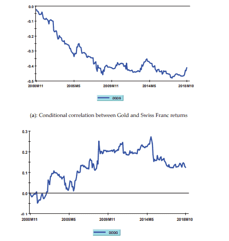
This section employs a well-known approach belonging to the class of Multivariate Garch estimators, namely Engle (2002) Dynamic Conditional Correlation model, in order to compute time-varying conditional correlations between asset returns. The first sub-section provides a short outline of this econometric framework. The latter sub-section presents parameters estimates and analyzes pair-wise correlation patterns between asset returns. 3.1. Engle (2002) Dynamic Conditional Correlation Model Let $r_{t}=\left(r_{1 t}, \ldots, r_{n t}\right)$ represent a $(n \times 1)$ vector of financial assets returns at time (t). Moreover, let $\varepsilon_{t}$ $=\left(\varepsilon_{1 t}, \ldots, \varepsilon_{n t}\right)$ be a $(n \times 1)$ vector of error terms obtained from an estimated system of mean equations for these return series.
Engle (2002) proposes the following decomposition for the conditional variance-covariance matrix of asset returns: $$ H_{t}=D_{t} R_{t} D_{t} $$ where $D_{t}$ is a $(n \times n)$ diagonal matrix of time-varying standard deviations from univariate Garch models, and $R_{t}$ is a $(n \times n)$ time-varying correlation matrix of asset returns $\left(\rho_{i j}, t\right)$.
The conditional variance-covariance matrix $\left(\mathrm{H}{t}\right)$ displayed in equation [1] is estimated in two steps. In the first step, univariate Garch $(1,1)$ models are applied to mean returns equations, thus obtaining conditional variance estimates for each financial asset ( $\sigma{i t}^{2} ;$ for $\left.i=1,2, \ldots ., n\right)$, namely: $$ \sigma_{i t}^{2}=\sigma_{U i t}^{2}\left(1-\lambda_{1 i}-\lambda_{2 i}\right)+\lambda_{1 i} \sigma_{i, t-1}^{2}+\lambda_{2 i} \varepsilon_{i, t-1}^{2} $$
where $\sigma^{2}$ uit is the unconditional variance of the $i$ th asset return, $\lambda_{1 i}$ is the volatility persistence parameter, and $\lambda_{2 i}$ is the parameter capturing the influence of past errors on the conditional variance. In the second step, the residuals vector obtained from the mean equations system $\left(\varepsilon_{t}\right)$ is divided by the corresponding estimated standard deviations, thus obtaining standardized residuals (i.e., $u_{i t}=$ $\varepsilon_{i t} / \sqrt{\sigma_{i, t}^{2}}$ for $\left.\mathrm{i}=1,2, \ldots ., n\right)$, which are subsequently used to estimate the parameters governing the time-varying correlation matrix.
More specifically, the dynamic conditional correlation matrix of asset returns may be expressed as: $$ Q_{t}=\left(1-\delta_{1}-\delta_{2}\right) \overline{\mathrm{Q}}+\delta_{1} Q_{t-1}+\delta_{2}\left(u_{t-1} u_{t-1}^{\prime}\right) $$ where $\overline{\mathrm{Q}}=\mathrm{E}\left[u_{t} u_{t}^{\prime}\right]$ is the $(n \times n)$ unconditional covariance matrix of standardized residuals, and $\delta_{1}$ and $\delta_{2}$ are parameters (capturing, respectively, the persistence in correlation dynamics and the impact of past shocks on current conditional correlations).
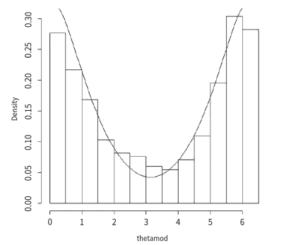
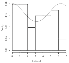
8.1. Inference on the Gold Price Data (In US Dollars) (1980-2013) Gold price data, say $x_{t}$, were collected per ounce in US dollars over the years $1980-2013 .$ These were transformed as $z_{t}=100\left(\ln \left(x_{t}\right)-\ln \left(x_{t-1}\right)\right)$, which were then “wrapped” to obtain $\theta_{t}=z_{t} \bmod 2 \pi$ and finally transformed to $\hat{\theta}=\left(\theta_{t}-\bar{\theta}\right) \bmod 2 \pi$, where $\bar{\theta}$ denotes the mean direction of $\theta_{t}$ and $\hat{\theta}$ denotes the variable thetamod as used in the graphs. The Durbin-Watson test performed on the log ratio transformed data shows that the autocorrelation is zero. The test statistic of Watson’s goodness of fit Jammalamadaka and SenGupta (2001) for wrapped stable distribution was obtained as $0.01632691$ and the corresponding P-value was obtained as $0.9970284$, which is greater than $0.05$, indicating that the wrapped stable distribution fits the transformed gold price data (in US dollars). The modified truncated estimate $\hat{\alpha}_{1}^{*}$ is $0.3752206$ while the estimate by characteristic function method is $0.401409$. The value of the objective function using the characteristic function estimate is $2.218941$ while that using our modified truncated estimate is $2.411018$. 8.2. Inference on the Silver Price Data (In US Dollars) (1980-2013) Data on the price of silver in US dollars collected per ounce over the same time period also underwent the same transformation. The Durbin-Watson test performed on the log ratio transformed data shows that the autocorrelation is zero. Here, the Watson’s goodness of fit test for wrapped stable distribution was also performed and the value of the statistic was obtained as $0.02530653$ and the corresponding $p$-value is $0.9639666$, which is greater than $0.05$, indicating that the wrapped stable distribution also fits the transformed silver price data (in US dollars). The modified truncated estimate of the index parameter $\alpha$ is $0.4112475$ while the estimate by characteristic function method is $0.644846 .$ The value of the objective function using the characteristic function estimate is $2.234203$ while that using our modified truncated estimate is $2.234432$.
统计代写|金融统计代写Financial Statistics代考|Findings and Concluding Remarks
It can be observed from Table 1 that the asymptotic variance of the untruncated estimator is reduced for the corresponding truncated estimator, indicating the efficiency of the truncated estimator. It can also be noted from Table 2 that, for $\alpha=1.01$, the RMSE of the modified truncated estimator is less than that of the Hill estimator when the sample is relocated by three different relocations, viz. true mean $=0$, sample mean, and sample median, for higher values of the concentration parameter $\rho=0.5,0.6,0.8$, and $0.9$ for sample sizes $n=100,250,500$, and 1000 and for $\rho=0.3,0.4,0.6,0.8$, and $0.9$ for sample sizes $n=2000,5000$, and 10,000 . Furthermore, it can be observed that, for $\alpha=1.25,1.5$, $1.75$ and 1.9, the RMSE of the modified truncated is less than that of the Hill estimator for different relocations for $\rho=0.6,0.7,0.8$, and $0.9$ for smaller sample size and even for $\rho=0.5$ for larger sample size. This clearly indicates the efficiency of the modified truncated estimator over the Hill estimator for higher values of the concentration parameter $\rho$.
It can be observed in Table 3 that the RMSE of the modified truncated estimator is less than that of the characteristic function-based estimator for almost all values of $\alpha$ corresponding to all values of $\sigma$. The Hill estimator (Dufour and Kurz-Kim $(2010)$ ) is defined for $1 \leq \alpha \leq 2$, whereas the modified truncated estimator is defined for the whole range $0 \leq \alpha \leq 2$. In addition, the overall performance of the modified truncated estimator is quite good in terms of efficiency and consistency over both the Hill estimator and the characteristic function-based estimator.
Thus, we have established an estimator of the index parameter $\alpha$ that strongly supports its parameter space $(0,2]$. It can be observed from the above real life data applications that the modified truncated estimator is quite close to that of the characteristic function-based estimator. In addition, it is simpler and computationally easier than that of the estimator defined in Anderson and Arnold (1993). Thus, it may be considered as a better estimator.
Again, when the estimator of $a$ lies between 1 and 2 , is attempted to model a mixture of two distributions with the value of the index parameter as that of the two extreme tails that is modeling a mixture of Cauchy $(\alpha=1)$ and normal $(\alpha=2)$ distributions when $1<\alpha<2$ or modeling a mixture of Double Exponential $\left(\alpha=\frac{1}{2}\right)$ and Cauchy $(\alpha=1)$ distributions when $\frac{1}{2}<\alpha<1$. Then, it is compared with that of the stable family of distributions for goodness of fit.
We could have used the usual technique of non-linear optimization as used in Salimi et al. (2018) for estimation, but it is computationally demanding and also the (statistical) consistency of the estimators obtained by such method is unknown. In contrast, our proposed methods of trigonometric moment and modified truncated estimation are much simpler, computationally easier and also possess useful consistency properties and, even their asymptotic distributions can be presented in simple and elegant forms as already proved above.
统计代写|金融统计代写Financial Statistics代考|Background
In this section we provide briefly some background on Markov chains and results on stationarity of PHARCH models. 2.1. Markoo Chains Suppose that $\mathbf{X}=\left{X_{n}, n \in \mathbb{Z}^{+}\right}, \mathbb{Z}^{+}:={0,1,2, \ldots}$ are random variables defined over $(\Omega, \mathcal{F}, \mathcal{B}(\Omega))$, and assume that $\mathrm{X}$ is a Markov chain with transition probability $P(x, A), x \in \Omega, A \subset \Omega$. Then we have the following definitions:
A function $f: \Omega \rightarrow \mathbb{R}$ is called the smallect semi-continuous function if $\liminf _{y \rightarrow x} f(y) \geq$ $f(x), x \in \Omega$. If $P(\cdot, A)$ is the smallest semi-continuous function for any open set $A \in \mathcal{B}(\Omega)$, we say that (the chain) $\mathbf{X}$ is a weak Feller chain.
A chain $\mathbf{X}$ is called $\varphi$-irreducible if there exists a measure $\varphi$ on $\mathcal{B}(\Omega)$ such that, for all $x$, whenever $\varphi(A)>0$, we have, $$ U(x, A)=\sum_{n=1}^{\infty} P^{n}(x, A)>0 . $$
The measure $\psi$ is called maximal with respect to $\varphi$, and we write $\psi>\varphi$, if $\psi(A)=0$ implies $\varphi(A)=0$, for all $A \in \mathcal{B}(\Omega)$. If $\mathbf{X}$ is $\varphi$-irreducible, then there exists a probability measure $\psi$, maximal, such that $\mathbf{X}$ is $\psi$-irreducible.
Let $d={d(n)}$ a distribution or a probability measure on $\mathbb{Z}^{+}$, and consider the Markov chain $\mathbf{X}{d}$ with transition kernel $$ K{d}(x, A):=\sum_{n=0}^{\infty} P^{n}(x, A) d(n) $$ If there exits a transition kernel $T$ satisfying $$ K_{d}(x, A) \geq T(x, A), \quad x \in \Omega, A \in \mathcal{B}(\Omega), $$ then $T$ is called the continuous component of $K_{d}$.
If $\mathbf{X}$ is a Markov chain for which there exits a (sample) distribution $d$ such that $K_{d}$ has a continuous component $T$, with $T(x, \Omega)>0, \forall x$, then $\mathbf{X}$ is called a $T$-chain.
A measure $\pi$ over $\mathcal{B}(\Omega), \sigma$-finite, with the property $$ \pi(A)=\int_{\Omega} \pi(d x) P(x, A), A \in \mathcal{B}(\Omega) $$ is called an invariant measure. The following two lemmas will be useful. See Meyn and Tweedie (1996) for the proofs and further details. We denote by $I_{A}(\cdot)$ the indicator function of $A$.
统计代写|金融统计代写Financial Statistics代考|The Trigonometric Moment Estimator
The regular symmetric stable distribution is defined through its characteristic function given by $$ \varphi(t)=\exp \left(i t \mu-|\sigma t|^{a}\right) $$ where $\mu$ is the location parameter; $\sigma$ is the scale parameter, which we take as 1; and $\alpha$ is the index or shape parameter of the distribution. Here, without loss of generality, we take $\mu=0$.
From the stable distribution, we can obtain the wrapped stable distribution (the process of wrapping explained in Jammalamadaka and SenGupta (2001)). Suppose $\theta_{1}, \theta_{2}, \ldots, \theta_{m}$ is a random sample of size $m$ drawn from the wrapped stable (given in Jammalamadaka and SenGupta (2001)) distribution whose probability density function is given by $$ f(\theta, \rho, a, \mu)=\frac{1}{2 \pi}\left[1+2 \sum_{p=1}^{\infty} \rho^{p^{n}} \cos p(\theta-\mu)\right] \quad 0<\rho \leq 1,0<\alpha \leq 2,0<\mu \leq 2 \pi $$ It is known in general from Jammalamadaka and SenGupta (2001) that the characteristic function of $\theta$ at the integer $p$ is defined as, $$ \psi_{\theta}(p)=E[\exp (i p(\theta-\mu))]=\alpha_{p}+i \beta_{p} $$ where $\quad a_{p}=E \cos p(\theta-\mu)$ and $\beta_{p}=E \sin p(\theta-\mu)$ Furthermore, from Jammalamadaka and SenGupta (2001), it is known that for, the p.d.f given by Equation (1), $$ \psi_{\theta}(p)=\rho^{p^{n}} $$ Hence, $E \cos p(\theta-\mu)=\rho^{p^{*}}$ and $E \sin p(\theta-\mu)=0$ We define $$ C_{1}=\frac{1}{m} \sum_{i=1}^{m} \cos \theta_{i}, \quad C_{2}=\frac{1}{m} \sum_{i=1}^{m} \cos 2 \theta_{i}, \quad S_{1}=\frac{1}{m} \sum_{i=1}^{m} \sin \theta_{i} $$ and $\quad \bar{S}{2}=\frac{1}{m} \sum{i=1}^{m} \sin 2 \theta_{i}$ Then, we note that $\bar{R}{1}=\sqrt{{\overline{C{1}}}^{2}+{\overline{S_{1}}}^{2}}$ and $\bar{R}{2}=\sqrt{{\overline{C{2}}}^{2}+\bar{S}_{2}^{2}}$
By the method of trigonometric moments estimation, equating $K_{1}$ and $R_{2}$ to the corresponding functions of the theoretical trigonometric moments, we get the estimator of index parameter $\alpha$ as (see SenGupta (1996)): $$ \hat{k}=\frac{1}{\ln 2} \ln \frac{\ln \bar{R}{2}}{\ln \bar{R}{1}} $$ Then, we define $\bar{R}{j}=\frac{1}{m} \sum{i=1}^{m} \cos j\left(\theta_{i}-\bar{\theta}\right), j=1,2$ and $\bar{\theta}$ is the mean direction given by $\bar{\theta}=\arctan \left(\frac{\xi_{1}}{C_{1}}\right)$. Note that $K_{1} \equiv R$. We consider two special cases.
统计代写|金融统计代写Financial Statistics代考|Improvement Over the Moment Estimator
The moment estimator need not always remain in the support of the true parameter $\alpha($ that is $(0,2])$. Hence, the moment estimators proposed above do not need to be proper estimators of $\alpha$. A modified estimator free from this defect is given by $$ \begin{aligned} \hat{a^{*}} &=\hat{u} \quad \text { if } 0<\hat{u}<2 \ &=2 \quad \text { if } \hat{a} \geq 2 \end{aligned} $$ (since support of $a$ excludes non-positive values). Thus, the density function of $\hat{\alpha}$ * is given by $$ \begin{aligned} g\left(\hat{a^{}}\right) &=\frac{P[\hat{a}<2]}{P[\hat{a} \geq 0]} \quad ; 0<\hat{a^{}}<2 \equiv-\infty<\hat{a}<2 \ &=P\left[\hat{a^{}}=2\right] \quad ; \hat{a^{}}=2 \equiv \hat{k} \geq 2 \ &=\frac{P[\hat{a} \geq 2]}{P[\hat{a} \geq 0]} \quad ; \hat{a^{}}=2 \equiv \hat{a} \geq 2 \end{aligned} $$ where $f(\hat{\alpha})$ is the density function of $\hat{k} \sim N(a, \gamma / \Sigma \gamma / m)$. Therefore, $g\left(\hat{\alpha}^{}\right)=\frac{\Phi\left(\frac{2-a}{\sqrt{I^{12} / m}}\right)}{1-\Phi\left(\frac{-a}{\sqrt{I^{2}-\sqrt{y}}}\right)} \quad ; 0<\hat{a^{}}<2 \equiv-\infty$ $=1-\frac{\Phi\left(\frac{2-a}{\sqrt{x^{12} y^{/ m}}}\right)}{\Phi\left(\frac{a}{\sqrt{I^{2}} y^{/ m}}\right)} ; \hat{x^{}}=2 \equiv \hat{k} \geq 2$ Thus, we get $g\left(\hat{\alpha}^{}\right)$ as a mixed distribution of one atomic mass function and a continuous function. 4.1. Special Case 1: $\mu=0, \sigma=1$ 4.2. Special Case 2 : $\mu=0, \sigma$ Lnknown Similar modifications can be made for the estimator ${\hat{\alpha_{2}}}^{\text {. }}$. Let it be denoted by $\hat{\alpha_{2}^{}}$.
统计代写|金融统计代写Financial Statistics代考|Derivation of the Asymptotic Distribution of the Modified Truncated Estimators
Now, using the asymptotic normal distribution of $\tilde{a}$, we can derive the same results for the modified truncated estimator of the index parameter $\alpha$ (given as below) as we have done for the method of moment estimator of $\alpha$. The mean of $\hat{a^{}}$ is given by $$ E\left(\hat{\alpha}^{}\right)=0 . P(\hat{a}<0)+\int_{0}^{2} \hat{\alpha} f(\hat{u}) d \hat{u}+2 \cdot P(\hat{a}>2) $$ where $\sqrt{m}(\hat{\alpha}-\alpha) \rightarrow \mathrm{N}\left(0, \underline{y}^{\prime} \underline{y}\right)$ asymptotically (as noted above) and $\mathrm{f}(\hat{\alpha})=$ probability density function of $\hat{a}$. The above is equivalent to $\tau=\frac{\frac{\pi-\pi}{\sqrt{y^{2} \gamma^{\prime m}}}}{}$ Let $\phi(\tau)$ and $\Phi(\tau)$ denote the p.d.f. and c.d.f. of $\tau$, respectively. Let $\sigma=\sqrt{\frac{m^{2}}{m}}$. Then, we get, $$ \begin{aligned} &E\left(\hat{\alpha}^{}\right)=a P\left(\tau}\right)+\int_{a^{}}^{b^{}}(\tau \sigma+\alpha) \phi(\tau) d \tau+b P\left(\tau>b^{}\right) \ &\Rightarrow E\left(\hat{\alpha}^{}\right)=\sigma\left[\left{\phi\left(a^{}\right)-\phi\left(b^{}\right)\right}\right]+\alpha\left[\Phi\left(b^{}\right)-\Phi\left(a^{}\right)\right] \end{aligned} $$ $=\alpha$ since $\left[\Phi\left(b^{}\right)-\Phi\left(a^{}\right)\right] \rightarrow 1, b\left[1-\Phi\left(b^{}\right)\right] \rightarrow 0$ and $\sigma \rightarrow 0$ as $m \rightarrow$ infinity where $a^{}=\frac{-a}{\sqrt{\frac{L^{2}}{m}}} \quad$ and $b^{}=\frac{2-\alpha}{\sqrt{\frac{\pi^{2}-y}{m}}}$ $E\left(\hat{\alpha}^{2}\right)=0^{2} \cdot P(\hat{\alpha}<0)+\int_{0}^{2} \hat{\alpha}^{2} f(\hat{\alpha}) \mathrm{d} \hat{\alpha}+4 \cdot P(\hat{\alpha}>2)$ $$ \Rightarrow E\left(\hat{a}^{2}\right)=\sigma^{2}\left[\left{a^{} \phi\left(a^{}\right)-b^{} \phi\left(b^{}\right)+\Phi\left(b^{}\right)-\Phi\left(a^{}\right)\right}\right]+\alpha^{2}\left{\Phi\left(b^{}\right)-\Phi\left(a^{}\right)\right}+2 \alpha \sigma\left{\phi\left(a^{}\right)-\right. $$ $\left.\phi\left(b^{}\right)\right}$ since $b^{2} .\left[1-\Phi\left(b^{\prime}\right)\right] \rightarrow 0$ as $m \rightarrow$ infinity The asymptotic variance of $\hat{\alpha^{}}$ is given by $$ V\left(\hat{\alpha^{}}\right)=E\left({\hat{a^{}}}^{2}\right)-\left[E\left(\hat{a}^{}\right)\right]^{2} $$ Similarly, the mean of $\hat{x_{1}^{}}$ is given by $$ \begin{gathered} E\left(\hat{a}{1}^{*}\right)=\frac{\left.\sigma \frac{\left(\partial y\left(T{m}^{\prime}\right)\right.}{d}\right)}{\sqrt{m}}\left[\left{\phi\left(a^{\prime}\right)-\phi\left(b^{\prime}\right)\right}\right]+\alpha\left[\Phi\left(b^{\prime}\right)-\Phi\left(a^{\prime}\right)\right] \text { since } b\left[1-\Phi\left(b^{\prime}\right)\right] \rightarrow 0 \text { as } m \rightarrow \text { infinity } \ E\left(\hat{a}{1}^{2}\right)=\frac{\left.\sigma^{2} \frac{\partial \partial\left(T{m}^{\prime}\right)}{\partial \mu^{\prime}}\right)^{2}}{m}\left[\left{a^{\prime} \phi\left(a^{\prime}\right)-b^{\prime} \phi\left(b^{\prime}\right)+\Phi\left(b^{\prime}\right)-\Phi\left(a^{\prime}\right)\right}\right]+\alpha^{2}\left{\Phi\left(b^{\prime}\right)-\Phi\left(a^{\prime}\right)\right}+ \ 2 \alpha \frac{\left.\sigma \frac{\left(d x\left(J_{m}^{\prime}\right)\right.}{d m}\right)}{\sqrt{m}}\left{\phi\left(a^{\prime}\right)-\phi\left(b^{\prime}\right)\right} \text { since } b^{2} \cdot\left[1-\Phi\left(b^{\prime}\right)\right] \rightarrow 0 \text { as } m \rightarrow \text { infinity } \end{gathered} $$
统计代写|金融统计代写Financial Statistics代考|Improvement Over the Moment Estimator
矩估计器不必总是保持在真实参数的支持下 $\alpha$ (那是 $(0,2])$. 因此,上面提出的矩估计量不需要是适当的估计量 $\alpha$. 没有这 个缺陷的修正估计量由下式给出 $$ \hat{a^{*}}=\hat{u} \quad \text { if } 0<\hat{u}<2 \quad=2 \quad \text { if } \hat{a} \geq 2 $$ (由于支持 $a$ 不包括非正值)。 因此,密度函数 $\hat{\alpha}^{\star}$ 是 (谁) 给的 $$ g(\hat{a})=\frac{P[\hat{a}<2]}{P[\hat{a} \geq 0]} \quad ; 0<\hat{a}<2 \equiv-\infty<\hat{a}<2 \quad=P[\hat{a}=2] \quad ; \hat{a}=2 \equiv \hat{k} \geq 2=\frac{P[\hat{a} \geq 2]}{P[\hat{a} \geq 0]} \quad ; \hat{a}= $$ 在哪里 $f(\hat{\alpha})$ 是 $\$$ \hat ${k} \backslash \operatorname{sim} N(a, \backslash$ Igamma / ISigma $\backslash$ 【gamma $/ m)$ 的密度函数. There fore, $\mathrm{~ g l l e f t ( ( h a t { a l p h a }}$ Isqrt{y}}}\right)} \quad ; $0<\backslash$ hat ${a \wedge{}}<2 \mathrm{~ l e q u i v – l i n f t y = 1 – I f r a c { 1 P h i l l e f t ( f r a c { 2 – a } {}$ $\left{\right.$ Phivleft(frac ${a}\left{\backslash \operatorname{sqrt}{\backslash \wedge{2}} \mathrm{~ y ^ { / ~}\right.$ gleft(Mhat{alpha}^{}〉right) asamixeddistributionofoneatomicmass functionandacontinuous function. 4.1.SpecialCase 1 : $\backslash \mathrm{mu}=0, \backslash$ |sigma $=14.2 .$ SpecialCase 2 : 亩 $=0$ , 西格玛 LnknownSimilarmodificationscanbemade fortheestimator ${$ hat ${$ alpha_{2}}} ${$ text ${.}}$ . Letitbedenotedby hat{lalpha_{2}^{}}\$
统计代写|金融统计代写Financial Statistics代考|Derivation of the Asymptotic Distribution of the Modified Truncated Estimators
现在,使用渐近正态分布 $\tilde{a}$ ,我们可以为索引参数的修改裁断估计推导出相同的结果 $\alpha$ (如下所示) 正如我们对矩估计的 方法所做的那样 $\alpha$. 的平均值 $\hat{a}$ 是 (谁) 给的 $$ E(\hat{\alpha})=0 . P(\hat{a}<0)+\int_{0}^{2} \hat{\alpha} f(\hat{u}) d \hat{u}+2 \cdot P(\hat{a}>2) $$ 其中 $\$ \backslash$ sqrt ${\mathrm{m}} \mathrm{~ ( ~ V h a t {}$ asymptotically(asnotedabove) and $\backslash$ mathrm ${f}($ hat ${\backslash a \mid p h a})=$ probabilitydensity functionof $\backslash$ 帞子 ${a}$ $.$ Theaboveisequivalentto $\backslash$ tau $=\backslash$ frac ${\backslash$ frac ${\backslash$ pi- $\backslash$ pi $}{\backslash$ sqrt ${\mathrm{y} \wedge{2} \backslash$ gamma $\wedge{\backslash \mathrm{~ p r i m e ~ m } } } } } L e t \ p h i (}$ and $\backslash$ 披(\tau)denotethep.d.f. andc. d. f.of $\backslash$ ⿶大 . respectively. Let $\backslash \mathrm{sigma}=\backslash \mathrm{sqrt}{\backslash \mathrm{frac}{\mathrm{m} \wedge{2}}{\mathrm{m}}}$ . Then, weget, $\mathrm{~ V b e g i n { 对 六 } ~ \& E : Y e f t ( N h a t { a l p h a } ^ { } l r i g h t ) = a ~ P}$ $=\backslash \mathrm{~ 阿 尔 法 s i n c e \ l e f t [ \ P h i ソ}$ \rightarrow $0 a n d \backslash$ sigma \rightarrow $0 a s \mathrm{~ 米 \ 右 箭 头 ~ i n ~ f i n i t y w h e r e a}$ and $\mathrm{b}^{\wedge}{}=\backslash$ frac ${2-\backslash a l p h a} \backslash s q r t{$ frac $\left.\left.{\mathrm{pi} \wedge{2}-\mathrm{y}} \mathrm{m}}\right}\right} \mathrm{E} \backslash$ eft(:hat ${\backslash a \mid p h a} \wedge{2} \backslash$ right) $=0 \wedge{2} \backslash \mathrm{cdot} \mathrm{P}(\backslash$ $$ V(\hat{\alpha})=E\left(\hat{a}^{2}\right)-[E(\hat{a})]^{2} $$ 同样,平肑值 $\hat{x_{1}}$ 是 (谁) 给的 $\mathrm{~ V b e g i n { 聚 隹 ~ E V}$
统计代写|金融统计代写Financial Statistics代考|Main aspects of integral model
The period of time for which the integral model is constructed, should consist of a few waves of the underwriting cycle. The integral model is multi-component. It includes a number of different partial models, with each different phase of the
cycle. Within each partial model, the specific behavior of the market as a whole and of the individual companies on it has its own internal reasons; its investigation will be our most important task.
Thus, we imbed the theory of competition-originated underwriting cycles into the general theory of complex reflexive systems. We emphasize the role of human error, and of incomplete understanding of the real market situation. Our challenge is the development of an integral model suitable for quantitative, rather than merely qualitative analysis.
Of particular interest to us are long-term strategies, rather than annual control decisions. This is because we cannot be sure that a growing company will not face solvency problems in the next few years, even though at present it successfully fulfills all solvency requirements set by the regulator. Moreover, the insolvency of such a company may be unexpected to an external observer, especially after growth in the volume of its business and its revenue for several years due to the influx of insurers. In other words, besides ruin within an insurance year, another threat is the inability to meet the minimum solvency requirements in the next new year $^{8}$, known as default. This threat is especially grave when a company grows, as the capital needed to maintain solvency may grow even faster than its revenues.
统计代写|金融统计代写Financial Statistics代考|Factors used in quantitative analysis
We have already discussed (see Section 1.4.4.1) the interconnection between underwriting cycles, price competition and migration of insureds. To continue, let us say that the insurers’ behavior on the competitive insurance market has internal causes linked with the following observations.
The insureds who desire to reduce their expenses may opt to switch insurer $^{9}$, which explains the possibility of business expansion by means of price cut amongst aggressive insurers. Besides that, on a profitable market, price cuts usually aim to show greater profit in the annual report; this is directly connected with income on equity. Therefore, a second factor is the desire of insurance managers to enhance the attractiveness of the company in the opinion of investors. Further, it is required (e.g., by regulation) to meet solvency requirements. In principle, managers are responsible not only for the current activity of the company, but for
its long-term survival. To protect insureds and creditors from the consequences of insolvency, all companies are inspected periodically by regulators, which keeps the competitive zeal of their managers in check.
For a quantitative analysis of rational strategies and internal causes of insurers” behavior in each partial model, we will consider the combined influence of three factors: Expansion, Revenue and Solvency. In [123], it is called $E R S$-analysis. It is consistent with the opinion of practitioners (see, e.g., [173]) and theorists (see, e.g., [102]) that since single-factorial approaches are unable to explain the real causes of underwriting cycles and crisis phenomena satisfactorily, multifactorial approaches should be applied instead.
In the following chapters, we will measure solvency in monetary units ${ }^{10}$ when performing quantitative $E R S$-analysis. To do this, we turn to the concept of nonruin capital which allows solvency to be annually maintained at a predetermined level. In Lundberg’s collective risk model (see Section 1.5.2), or in the diffusion risk model (see Section 1.5.4), the non-ruin capital is defined as a solution to a nonlinear equation, in which the left-hand side is the probability of ruin within finite time, and the right-hand side is the small number $\alpha \in(0,1)$, i.e., the predetermined solvency’s level. The non-ruin capital is harder to evaluate than the probability of ruin, but its use makes $E R S$-analysis more intuitive and instructive.
统计代写|金融统计代写Financial Statistics代考|Driving forces behind the cycles and two main causal connections
The casualties of misfortune, accidental errors, stubbornness of some shareholders, or a reluctance of managers to follow good advices are hardly among the main
driving forces of underwriting cycles ${ }^{15}$. These real driving forces come from the difference between the market participants’ interests. On the profitable market, the typical interest of
a company which recently entered the market is the growth of its business. Such a growth-seeking company is often impelled, regardless of potential loss, to resort to price cut to attract new customers. This move is not illegal in itself. However, it can lead to cumulative errors in the company’s assessment of its long-term financial strength. For an aggressive company, the main mistake in the perception of reality lies usually in inaccurate evaluation, or in neglecting the evaluation, of its own solvency. The negative consequences of these errors are most fully manifested when the profitableness of the market falls;
an incumbent company that has a large portfolio is getting stable profit from conducting regular insurance operations. But this business goal of a profitseeking company can sometimes be achieved through indirect means. For example, wanting to force the aggressive newcomers to change their goal to profit-seeking, the incumbent company may resort to a reduction of its own prices. Such sacrifice of possible income, an unnatural move on the market without competition, is an instrument for protecting a position on the market with growing competition;
a company that tries to take immediate advantage of the current situation is using any chance to increase its volume and income, as circumstances permit. This pursuit of mercantile interests sometimes leads the opportunistic company to undertake a mercenary behavior.