如果你也在 怎样代写金融统计Financial Statistics这个学科遇到相关的难题,请随时右上角联系我们的24/7代写客服。
金融统计是将经济物理学应用于金融市场。它没有采用金融学的规范性根源,而是采用实证主义框架。它包括统计物理学的典范,强调金融市场的突发或集体属性。经验观察到的风格化事实是这种理解金融市场的方法的出发点。
statistics-lab™ 为您的留学生涯保驾护航 在代写金融统计Financial Statistics方面已经树立了自己的口碑, 保证靠谱, 高质且原创的统计Statistics代写服务。我们的专家在代写金融统计Financial Statistics代写方面经验极为丰富,各种代写金融统计Financial Statistics相关的作业也就用不着说。
我们提供的金融统计Financial Statistics及其相关学科的代写,服务范围广, 其中包括但不限于:
- Statistical Inference 统计推断
- Statistical Computing 统计计算
- Advanced Probability Theory 高等概率论
- Advanced Mathematical Statistics 高等数理统计学
- (Generalized) Linear Models 广义线性模型
- Statistical Machine Learning 统计机器学习
- Longitudinal Data Analysis 纵向数据分析
- Foundations of Data Science 数据科学基础
统计代写|金融统计代写Financial Statistics代考|High Frequency Data
In this section we further elaborate on high frequency data and introduce the series that will be analyzed later. High frequency data are very important in the financial environment, mainly because there exist large movements in short intervals of time. This aspect represents an interesting opportunity for trading. Furthermore, it is well known that volatilities in different frequencies have significant cross-correlation. We can even say that coarse volatility predicts fine volatility better than the inverse, as shown in Dacorogna et al. (2001).
As an example, take the tick by tick foreign exchange (FX) time series Euro-Dollar, from January First 1999 to December 31, 2002. Returns are calculated using bid and ask prices, as
$$
r_{t}=\ln \left(\left(p_{t}^{b i d}+p_{t}^{a s k}\right) / 2\right)-\ln \left(\left(p_{t-1}^{b i d}+p_{t-1}^{a s k}\right) / 2\right)
$$
We discard Saturdays and Sundays, and we replace holidays with the means of the last ten observations of the returns for each respective hour and day. After cleaning the data (see Dacorogna et al. (2001), for details) we will consider equally spaced returns, with sampling interval $\Delta t=15 \mathrm{~min}$. This seems to be adequate, as many studies indicate.
Figure 2 shows Euro-Dollar returns calculated as above. The length of this time series is 95,317 . The figure shows that the absolute returns present a seasonal pattern. This is due to the fact that physical time does not follow, necessarily, the same pattern as the business time. This is a typical behavior of a financial time series and we will use a seasonal adjustment procedure similar to that of Martens et al. (2002). However, we will use absolute returns instead of squared returns; that is, we will compute the seasunal patturn as
$$
S_{d_{,}, h}=\frac{1}{s} \sum_{j=1}^{s} \mid\left(r_{d_{t}, j, t} \mid,\right.
$$
where $r_{d, s, t}$ is the return in the weekday $d$, week $s$ and hour $h$, and $s$ is the number of weeks from the beginning of the series. Therefore, $S_{d, N}, N_{t}$ is the rolling window mean of the absolute returns with the beginning fixed.
In Figure 3 we have the autocorrelation function of these returns and of squared returns. The seasonality pattern is no longer present.
FX data has some distinct characteristics, mainly because they are produced twenty four hours a day, seven days a week. In particular, Euro-Dollar is the most liquid FX in the world. However, there are periods where the activity is greater or smaller, causing seasonal patterns to occur, as seen above.
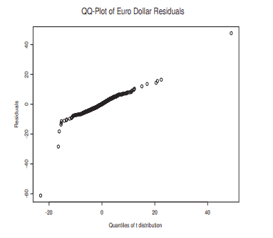
Let us analyze some facts about these returns that we will denote simply by rt. We can see in Figure 4 the histogram fitted with a non-parametric density kernel estimate, using unbiased cross-validation method to estimate the bandwidth. It shows fat tails and high kurtosis, namely, 121 , while its skewness coefficient is $-0.079$, showing almost symmetry. A normality test (Jarque-Bera) rejects the hypothesis that these returns are normal.
统计代写|金融统计代写Financial Statistics代考|Introduction and Motivation
A financial asset is referred to as a “safe haven” asset if it provides hedging benefits during periods of market turbulence. In other words, during periods of market stress, “safe haven” assets are supposed to be uncorrelated, or negatively correlated, with large markets slumps experienced by more traditional financial assets (typically stock or bond prices).
The financial literature identifies various asset classes exhibiting “safe haven” features: gold and other precious metals, the exchange rates of some key international currencies against the US dollar, oil and other important agricultural commodities, and US long-term government bonds.
This paper contributes to the existing literature focusing on some of the most representative “safe haven” assets, namely gold, the Swiss Franc/US dollar exchange rate, and oil. The main motivation behind this choice is twofold.
First, empirical research on these assets have attracted major attention in recent years, both from academia and from institutional investors. Second, there are some weaknesses in the applied literature that need to be addressed.
The hedging properties of gold and its monetary role as a store of value are widely documented. Jaffe $(1989)$ and Chua et al. (1990) find that gold yields significant portfolio diversification benefits. Moreover, the “safe haven” properties of gold in volatile market conditions are widely documented: See, among others, Baur and McDermott (2010), Hood and Malik (2013), Reboredo (2013), and Ciner et al. (2013).
The popular views of gold as a store of value and a “safe haven” asset are well described in Baur and McDermott (2010). As reported by these authors, the 17 th Century British Mercantilist Sir William Petty described gold as “wealth at all times and all places” (Petty 1690). This popular perception of gold spreads over centuries, reinforced by its historic links to money, and even today gold is described as “ant attractive each way bet” against risks of financial losses or inflation (Economist 2005, 2009).
Turning to the role of the Swiss Franc as a “safe haven” asset, Ranaldo and Söderlind (2010) documented that the Swiss currency yields substantial hedging benefits against a decrease in US stock prices and an increase in forex volatility. These findings corroborate earlier results (Kugler and Weder 2004; Campbell et al. 2010). More recent research documented that increased risk aversion after the 2008 global financial turmoil strengthened the “safe haven” role of the Swiss currency (Tamakoshi and Hamori 2014).
统计代写|金融统计代写Financial Statistics代考|A Multivariate Garch Model of Asset Returns
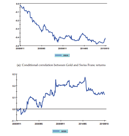
This section employs a well-known approach belonging to the class of Multivariate Garch estimators, namely Engle (2002) Dynamic Conditional Correlation model, in order to compute time-varying conditional correlations between asset returns. The first sub-section provides a short outline of this econometric framework. The latter sub-section presents parameters estimates and analyzes pair-wise correlation patterns between asset returns.
3.1. Engle (2002) Dynamic Conditional Correlation Model
Let $r_{t}=\left(r_{1 t}, \ldots, r_{n t}\right)$ represent a $(n \times 1)$ vector of financial assets returns at time (t). Moreover, let $\varepsilon_{t}$ $=\left(\varepsilon_{1 t}, \ldots, \varepsilon_{n t}\right)$ be a $(n \times 1)$ vector of error terms obtained from an estimated system of mean equations for these return series.
Engle (2002) proposes the following decomposition for the conditional variance-covariance matrix of asset returns:
$$
H_{t}=D_{t} R_{t} D_{t}
$$
where $D_{t}$ is a $(n \times n)$ diagonal matrix of time-varying standard deviations from univariate Garch models, and $R_{t}$ is a $(n \times n)$ time-varying correlation matrix of asset returns $\left(\rho_{i j}, t\right)$.
The conditional variance-covariance matrix $\left(\mathrm{H}{t}\right)$ displayed in equation [1] is estimated in two steps. In the first step, univariate Garch $(1,1)$ models are applied to mean returns equations, thus obtaining conditional variance estimates for each financial asset ( $\sigma{i t}^{2} ;$ for $\left.i=1,2, \ldots ., n\right)$, namely:
$$
\sigma_{i t}^{2}=\sigma_{U i t}^{2}\left(1-\lambda_{1 i}-\lambda_{2 i}\right)+\lambda_{1 i} \sigma_{i, t-1}^{2}+\lambda_{2 i} \varepsilon_{i, t-1}^{2}
$$
where $\sigma^{2}$ uit is the unconditional variance of the $i$ th asset return, $\lambda_{1 i}$ is the volatility persistence parameter, and $\lambda_{2 i}$ is the parameter capturing the influence of past errors on the conditional variance.
In the second step, the residuals vector obtained from the mean equations system $\left(\varepsilon_{t}\right)$ is divided by the corresponding estimated standard deviations, thus obtaining standardized residuals (i.e., $u_{i t}=$ $\varepsilon_{i t} / \sqrt{\sigma_{i, t}^{2}}$ for $\left.\mathrm{i}=1,2, \ldots ., n\right)$, which are subsequently used to estimate the parameters governing the time-varying correlation matrix.
More specifically, the dynamic conditional correlation matrix of asset returns may be expressed as:
$$
Q_{t}=\left(1-\delta_{1}-\delta_{2}\right) \overline{\mathrm{Q}}+\delta_{1} Q_{t-1}+\delta_{2}\left(u_{t-1} u_{t-1}^{\prime}\right)
$$
where $\overline{\mathrm{Q}}=\mathrm{E}\left[u_{t} u_{t}^{\prime}\right]$ is the $(n \times n)$ unconditional covariance matrix of standardized residuals, and $\delta_{1}$ and $\delta_{2}$ are parameters (capturing, respectively, the persistence in correlation dynamics and the impact of past shocks on current conditional correlations).
金融统计代考
统计代写|金融统计代写Financial Statistics代考|High Frequency Data
在本节中,我们将进一步阐述高频数据,并介绍稍后将要分析的系列。高频数据在金融环境中非常重要,主要是因为在 很短的时间间隔内存在较大的变动。䢒方面代表了一个有趣的交易机会。此外,众所周知,不同频率的波动率具有显着 的互相关性。我们甚至可以说,粗波动率比反之更能预测精细波动率,如 Dacorogna 等人所示。(2001 年)。
举个例子,从 1999 年 1 月 1 日到 2002 年 12 月 31 日,以逐笔交易 (FX) 时间序列欧元-美元为例。收益是使用买入价和 㛑出价计算得出的,如
$$
r_{t}=\ln \left(\left(p_{t}^{b i d}+p_{t}^{a s k}\right) / 2\right)-\ln \left(\left(p_{t-1}^{\text {bid }}+p_{t-1}^{a s k}\right) / 2\right)
$$
我们舍弃了周六和周日,我们用每个小时和一天的最后十次观䕓结果的平均值来代芘假期。清理数据后(详见 Dacorogna et al. (2001)),我们将考虑等距回报,采样间隔 $\Delta t=15 \mathrm{~min}$. 正如许多研究表明的那样,这似乎是足够 的。
图 2 显示了如上计算的欧元-美元回报。这个时间序列的长度是 95,317 。该图显示,绝对收益呈现䏮节性模式。这是因 $\mathrm{~ 为 物 理 时 间 不 一 定 遉 唕 与 业 务 时 间 相 同 的 模 式 。 这 是 金 融 时 间 序 列 的 典 型 行 为 , 我 们 将 使 用 类 似 于 ~ M a r t e n s ~ 等 人 的 曺}$ 性调整程序。(2002 年)。但是,我们将使用绝对收益而不是平方收益;也就是说,我们将计算季节性模式为
$$
S_{d, h}=\frac{1}{s} \sum_{j=1}^{s} \mid\left(r_{d_{t}, j, t} \mid\right.
$$
在哪里 $r_{d, s, t}$ 是工作日的回报 $d$ ,星期 $s$ 和小时 $h ,$ 和 $s$ 是从系列开始的周数。所以, $S_{d, N}, N_{t}$ 是开始固定的绝对收益的滚 动䆬口平均值。
在图 3 中,我们有这些回报和平方回报的自相关函数。录节性模式不再存在。
外汇数据有一些明显的特点,主要是因为它们是每周 7 天、每天 24 小时产生的。特别是,欧元美元是世界上流动性最强 的外汇。但是,如上所示,在某些时期活动更大或更小,导致出现季节性模式。
让我们分析一些关于这些收益的事实,我们将简单地用 rt 表示。我们可以在图 4 中看到拟合了非参数密度核估计的直方 图,使用无偏交叉验证方法来估计带宽。它显示出肥尾和高峰态,即 121 ,而其偏度系数为 $-0.079$ ,显示几平对称。 正态性检验 (Jarque-Bera) 拒绝这些回报是正常的假设。
统计代写|金融统计代写Financial Statistics代考|Introduction and Motivation
如果金融资产在市场动荡期间提供对冲收益,则该金融资产被称为“避风港”资产。换句话说,在市场压力期间,”避风港” 次产应该是不相关或负相关的,与更传统的金融资产(通常是股票或债券价格)经历的大市场晎跌。
金融文献确定了具有“避风港”特征的各种资产类别:黄金和其他贵金属、一些主要国际货市对美元的汇率、石油和其他重 要农产品,以及美国长期政府债券。
本文有助于现有文献关注一些最具代表性的”避风港”资产,即黄金、瑞士法郎/美元汇率和石油。这种选择背后的主要动 机是双重的。
首先,近年来对这些资产的实证研究引起了学术界和机构投资者的广泛关注。其次,应用文献中存在一些需要解决的弱 낸。
黄金的对冲属性及其作为价值储存手段的货币作用已被广泛记录。垔菲 $(1989)$ 和 Chua 等人。(1990) 发现黄金产生了显 着的投资组合多样化收益。此外,在波动的市场条件下,黄金的“避风港”属性已被广泛记录:参见 Baur 和 McDermott (2010 年)、Hood 和 Malik(2013 年) 、Reboredo(2013 年) 和 Ciner 等人。(2013)。
Baur 和 McDermott (2010) 很好地描述了黄金作为价值储存和”避风港”盗产的流行观点。正如这些作者所报道的那样, 17 世纪的英国重商主义者威廉·㑉蒂爵士将黄金描述为“随时随地的财富”(佩蒂 1690 年)。这种对黄金的普遍看法传播 了几个世纪,并因其与货币的历史联系而得到加强,即使在今天,黄金也被描述为“对金融损失或通货膨胀风险进行”单向 押注” (Economist 2005, 2009)。
谈到瑞士法郎作为”避风港”资产的作用,Ranaldo 和 Söderlind (2010) 证明,瑞士货币在美国股票价格下跌和外汇波动 性增加的情况下产生了巨大的对冲收益。这些发现证实了早期的结果 (Kugler 和 Weder 2004; Campbell 等人 2010)。最近的研究表明,在 2008 年全球金融动荡之后,风险厌恶情绪的增加加强了瑞士货市的“避风港”作用 (Tamakoshi 和 Hamori,2014 年)。
统计代写|金融统计代写Financial Statistics代考|A Multivariate Garch Model of Asset Returns
本节釆用属于多元 Garch 估计器爫的若名方法,即 Engle (2002) 动态条件相关模型,以计算资产收益之间的时变条件相 关性。第一个小节简要介绍了这个计量经济学框架。后面的小节介绍了参数估计并分析了资产回报之间的成对相关模 式。
3.1。Engle (2002) 动态条件相关模型
让 $r_{t}=\left(r_{1 t}, \ldots, r_{n t}\right)$ 代表一个 $(n \times 1)$ 时间 $(\mathrm{t})$ 的金融资产回报向量。此外,让 $\varepsilon_{t}=\left(\varepsilon_{1 t}, \ldots, \varepsilon_{n t}\right)$ 做一个 $(n \times 1)$ 从这些回报序列的估计平均方程系统获得的误差项向量。
Engle (2002) 对资产收益的条件方差-协方差矩阵提出了以下分解:
$$
H_{t}=D_{t} R_{t} D_{t}
$$
在哪里 $D_{t}$ 是一个 $(n \times n)$ 来自单变量 Garch 模型的时变标准差的对角矩阵,以及 $R_{t}$ 是一个 $(n \times n)$ 资产收益的时变相 关矩阵 $\left(\rho_{i j}, t\right)$.
条件方差-协方差矩阵 $(\mathrm{H} t)$ 等式 [1] 中显示的估计分两个步骤。第一步,单变量 $\operatorname{Garch}(1,1)$ 模型应用于平均收益方程, 从而获得每个金融资产的条件方差估计 $\left(\sigma i t^{2}\right.$; 为了 $\left.i=1,2, \ldots, n\right)$ ,即:
$$
\sigma_{i t}^{2}=\sigma_{U i t}^{2}\left(1-\lambda_{1 i}-\lambda_{2 i}\right)+\lambda_{1 i} \sigma_{i, t-1}^{2}+\lambda_{2 i} \varepsilon_{i, t-1}^{2}
$$
在哪里 $\sigma^{2}$ uit 是无条件方差 i资产回报率, $\lambda_{1 i}$ 是波动率持久性参数,并且 $\lambda_{2 i}$ 是捕捉过去误差对条件方差的影响的参数。 第二步,从均值方程组得到的残差向量 $\left(\varepsilon_{t}\right)$ 除以相应的估计标准差,从而获得标准化残差 (即, $u_{i t}=\varepsilon_{i t} / \sqrt{\sigma_{i, t}^{2}}$ 为了 $\mathrm{i}=1,2, \ldots, n)$, 随后用于估计控制时变相关矩阵的参数。
更具体地说,盗产收益的动态条件相关矩阵可以表示为:
$$
Q_{t}=\left(1-\delta_{1}-\delta_{2}\right) \overline{\mathrm{Q}}+\delta_{1} Q_{t-1}+\delta_{2}\left(u_{t-1} u_{t-1}^{\prime}\right)
$$
在哪里 $\overline{\mathrm{Q}}=\mathrm{E}\left[u_{t} u_{t}^{\prime}\right]$ 是个 $(n \times n)$ 标准化残差的无条件协方差矩阵,以及 $\delta_{1}$ 和 $\delta_{2}$ 是参数(分别捕获相关动态的持续性 和过去冲击对当前条件相关性的影响 $)$ 。

统计代写请认准statistics-lab™. statistics-lab™为您的留学生涯保驾护航。
金融工程代写
金融工程是使用数学技术来解决金融问题。金融工程使用计算机科学、统计学、经济学和应用数学领域的工具和知识来解决当前的金融问题,以及设计新的和创新的金融产品。
非参数统计代写
非参数统计指的是一种统计方法,其中不假设数据来自于由少数参数决定的规定模型;这种模型的例子包括正态分布模型和线性回归模型。
广义线性模型代考
广义线性模型(GLM)归属统计学领域,是一种应用灵活的线性回归模型。该模型允许因变量的偏差分布有除了正态分布之外的其它分布。
术语 广义线性模型(GLM)通常是指给定连续和/或分类预测因素的连续响应变量的常规线性回归模型。它包括多元线性回归,以及方差分析和方差分析(仅含固定效应)。
有限元方法代写
有限元方法(FEM)是一种流行的方法,用于数值解决工程和数学建模中出现的微分方程。典型的问题领域包括结构分析、传热、流体流动、质量运输和电磁势等传统领域。
有限元是一种通用的数值方法,用于解决两个或三个空间变量的偏微分方程(即一些边界值问题)。为了解决一个问题,有限元将一个大系统细分为更小、更简单的部分,称为有限元。这是通过在空间维度上的特定空间离散化来实现的,它是通过构建对象的网格来实现的:用于求解的数值域,它有有限数量的点。边界值问题的有限元方法表述最终导致一个代数方程组。该方法在域上对未知函数进行逼近。[1] 然后将模拟这些有限元的简单方程组合成一个更大的方程系统,以模拟整个问题。然后,有限元通过变化微积分使相关的误差函数最小化来逼近一个解决方案。
tatistics-lab作为专业的留学生服务机构,多年来已为美国、英国、加拿大、澳洲等留学热门地的学生提供专业的学术服务,包括但不限于Essay代写,Assignment代写,Dissertation代写,Report代写,小组作业代写,Proposal代写,Paper代写,Presentation代写,计算机作业代写,论文修改和润色,网课代做,exam代考等等。写作范围涵盖高中,本科,研究生等海外留学全阶段,辐射金融,经济学,会计学,审计学,管理学等全球99%专业科目。写作团队既有专业英语母语作者,也有海外名校硕博留学生,每位写作老师都拥有过硬的语言能力,专业的学科背景和学术写作经验。我们承诺100%原创,100%专业,100%准时,100%满意。
随机分析代写
随机微积分是数学的一个分支,对随机过程进行操作。它允许为随机过程的积分定义一个关于随机过程的一致的积分理论。这个领域是由日本数学家伊藤清在第二次世界大战期间创建并开始的。
时间序列分析代写
随机过程,是依赖于参数的一组随机变量的全体,参数通常是时间。 随机变量是随机现象的数量表现,其时间序列是一组按照时间发生先后顺序进行排列的数据点序列。通常一组时间序列的时间间隔为一恒定值(如1秒,5分钟,12小时,7天,1年),因此时间序列可以作为离散时间数据进行分析处理。研究时间序列数据的意义在于现实中,往往需要研究某个事物其随时间发展变化的规律。这就需要通过研究该事物过去发展的历史记录,以得到其自身发展的规律。
回归分析代写
多元回归分析渐进(Multiple Regression Analysis Asymptotics)属于计量经济学领域,主要是一种数学上的统计分析方法,可以分析复杂情况下各影响因素的数学关系,在自然科学、社会和经济学等多个领域内应用广泛。
MATLAB代写
MATLAB 是一种用于技术计算的高性能语言。它将计算、可视化和编程集成在一个易于使用的环境中,其中问题和解决方案以熟悉的数学符号表示。典型用途包括:数学和计算算法开发建模、仿真和原型制作数据分析、探索和可视化科学和工程图形应用程序开发,包括图形用户界面构建MATLAB 是一个交互式系统,其基本数据元素是一个不需要维度的数组。这使您可以解决许多技术计算问题,尤其是那些具有矩阵和向量公式的问题,而只需用 C 或 Fortran 等标量非交互式语言编写程序所需的时间的一小部分。MATLAB 名称代表矩阵实验室。MATLAB 最初的编写目的是提供对由 LINPACK 和 EISPACK 项目开发的矩阵软件的轻松访问,这两个项目共同代表了矩阵计算软件的最新技术。MATLAB 经过多年的发展,得到了许多用户的投入。在大学环境中,它是数学、工程和科学入门和高级课程的标准教学工具。在工业领域,MATLAB 是高效研究、开发和分析的首选工具。MATLAB 具有一系列称为工具箱的特定于应用程序的解决方案。对于大多数 MATLAB 用户来说非常重要,工具箱允许您学习和应用专业技术。工具箱是 MATLAB 函数(M 文件)的综合集合,可扩展 MATLAB 环境以解决特定类别的问题。可用工具箱的领域包括信号处理、控制系统、神经网络、模糊逻辑、小波、仿真等。