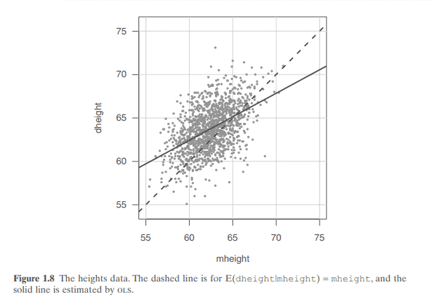
Imagine a generic summary plot of $Y$ versus $X$. Our interest centers on how the distribution of $Y$ changes as $X$ is varied. One important aspect of this distribution is the mean function, which we define by $$ \mathrm{E}(Y \mid X=x)=\text { a function that depends on the value of } x $$ We read the left side of this equation as “the expected value of the response when the predictor is fixed at the value $X=x$ “; if the notation ” $\mathrm{E}(\mathrm{)}$ ” for expectations and “Var( )” for variances is unfamiliar, refer to Appendix A.2. The right side of (1.1) depends on the problem. For example, in the heights data in Example 1.1, we might believe that $$ \mathrm{E}(\text { dheightlmheight }=x)=\beta_0+\beta_1 x $$ that is, the mean function is a straight line. This particular mean function has two parameters, an intercept $\beta_0$ and a slope $\beta_1$. If we knew the values of the $\beta \mathrm{s}$, then the mean function would be completely specified, but usually the $\beta \mathrm{s}$ need to be estimated from data. These parameters are discussed more fully in the next chapter.
Figure 1.8 shows two possibilities for the $\beta \mathrm{s}$ in the straight-line mean function (1.2) for the heights data. For the dashed line, $\beta_0=0$ and $\beta_1=1$. This mean function would suggest that daughters have the same height as their mothers on the average for mothers of any height. The second line is estimated using ordinary least squares, or ols, the estimation method that will be described in the next chapter. The ols line has slope less than 1 , meaning that tall mothers tend to have daughters who are taller than average because the slope is positive, but shorter than themselves because the slope is less than 1. Similarly, short mothers tend to have short daughters but taller than themselves. This is perhaps a surprising result and is the origin of the term regression, since extreme values in one generation tend to revert or regress toward the population mean in the next generation (Galton, 1886).
Another characteristic of the distribution of the response given the predictor is the variance function, defined by the symbol $\operatorname{Var}(Y \mid X=x)$ and in words as the variance of the response given that the predictor is fixed at $X=x$. For example, in Figure 1.2 we can see that the variance function for dheightlmheight is approximately the same for each of the three values of mheight shown in the graph. In the smallmouth bass data in Figure 1.5, an assumption that the variance is constant across the plot is plausible, even if it is not certain (see Problem 1.2). In the turkey data, we cannot say much about the variance function from the summary plot because we have plotted treatment means rather than the actual pen values, so the graph does not display the information about the variability between pens that have a fixed value of Dose.
A frequent assumption in fitting linear regression models is that the variance function is the same for every value of $x$. This is usually written as $$ \operatorname{Var}(Y \mid X=x)=\sigma^2 $$ where $\sigma^2$ (read “sigma squared”) is a generally unknown positive constant.
想象一下$Y$和$X$的一般汇总图。我们的兴趣集中在$Y$的分布如何随着$X$的变化而变化。这个分布的一个重要方面是均值函数,我们用 $$ \mathrm{E}(Y \mid X=x)=\text { a function that depends on the value of } x $$ 我们将这个方程的左边解读为“当预测器固定在$X=x$值时响应的期望值”;如果不熟悉表示期望的“$\mathrm{E}(\mathrm{)}$”和表示方差的“Var()”,请参阅附录A.2。(1.1)的右边取决于问题。例如,在例1.1中的高度数据中,我们可能认为 $$ \mathrm{E}(\text { dheightlmheight }=x)=\beta_0+\beta_1 x $$ 也就是说,均值函数是一条直线。这个特殊的平均函数有两个参数,一个截距$\beta_0$和一个斜率$\beta_1$。如果我们知道$\beta \mathrm{s}$的值,那么均值函数将被完全指定,但通常需要从数据中估计$\beta \mathrm{s}$。这些参数将在下一章中进行更详细的讨论。
This graduate level course offers an introduction into regression analysis. A Credits 3 researcher is often interested in using sample data to investigate relationships, with an ultimate goal of creating a model to predict a future value for some dependent variable. The process of finding this mathematical model that best fits the data involves regression analysis. STAT 501 is an applied linear regression course that emphasizes data analysis and interpretation. Generally, statistical regression is collection of methods for determining and using models that explain how a response variable (dependent variable) relates to one or more explanatory variables (predictor variables).
PREREQUISITES
This graduate level course covers the following topics:
Understanding the context for simple linear regression.
How to evaluate simple linear regression models
How a simple linear regression model is used to estimate and predict likely values
Understanding the assumptions that need to be met for a simple linear regression model to be valid
How multiple predictors can be included into a regression model
Understanding the assumptions that need to be met when multiple predictors are included in the regression model for the model to be valid
How a multiple linear regression model is used to estimate and predict likely values
Understanding how categorical predictors can be included into a regression model
How to transform data in order to deal with problems identified in the regression model
Strategies for building regression models
Distinguishing between outliers and influential data points and how to deal with these
Handling problems typically encountered in regression contexts
Alternative methods for estimating a regression line besides using ordinary least squares
Understanding regression models in time dependent contexts
Understanding regression models in non-linear contexts
Use the cig_1st_diff data set. This is based on the changes from 1990 to 2000 , and it is extracted from the data set used in Question #3. Estimate a first-difference model, as follows: regress cigch on taxch, uratech, and beertaxch. Weight the model by pop 2000 , and use robust standard errors. Interpret the estimate on taxch.
问题 2.
From the example in Section 8.5 from Card and Krueger (1994) on estimating the effects of minimum-wage increases on employment, write out the regression equation for the difference-in-difference model.
问题 3.
Use the data set oecd_gas_demand. From Question #7 in Chapter 3, add fixed effects for the country, along with a heteroskedasticity correction. a. How does the coefficient estimate on lrpmg change from Question #7 in Chapter 3 with the fixed effects added? b. How does this change which observations are compared to which observations?
问题 4.
Return to the tv-bmi-ecls data set used for Exercise $# 5$ in Chapter 6 . From that exercise, along with other descriptions of the research issue, there is much potential omitted-factors bias. a. Explore the data description and variable list (from the file “Exercises data set descriptions” on the book’s website). Design a model to address the omitted-factors bias. b. Are there any shortcomings to your approach?
Textbooks
• An Introduction to Stochastic Modeling, Fourth Edition by Pinsky and Karlin (freely available through the university library here) • Essentials of Stochastic Processes, Third Edition by Durrett (freely available through the university library here) To reiterate, the textbooks are freely available through the university library. Note that you must be connected to the university Wi-Fi or VPN to access the ebooks from the library links. Furthermore, the library links take some time to populate, so do not be alarmed if the webpage looks bare for a few seconds.
This graduate level course offers an introduction into regression analysis. A Credits 3 researcher is often interested in using sample data to investigate relationships, with an ultimate goal of creating a model to predict a future value for some dependent variable. The process of finding this mathematical model that best fits the data involves regression analysis. STAT 501 is an applied linear regression course that emphasizes data analysis and interpretation. Generally, statistical regression is collection of methods for determining and using models that explain how a response variable (dependent variable) relates to one or more explanatory variables (predictor variables).
PREREQUISITES
This graduate level course covers the following topics:
Understanding the context for simple linear regression.
How to evaluate simple linear regression models
How a simple linear regression model is used to estimate and predict likely values
Understanding the assumptions that need to be met for a simple linear regression model to be valid
How multiple predictors can be included into a regression model
Understanding the assumptions that need to be met when multiple predictors are included in the regression model for the model to be valid
How a multiple linear regression model is used to estimate and predict likely values
Understanding how categorical predictors can be included into a regression model
How to transform data in order to deal with problems identified in the regression model
Strategies for building regression models
Distinguishing between outliers and influential data points and how to deal with these
Handling problems typically encountered in regression contexts
Alternative methods for estimating a regression line besides using ordinary least squares
Understanding regression models in time dependent contexts
Understanding regression models in non-linear contexts
Indicate which of the four main regression objectives each of the following research issues would be: a. What 4th-grade teacher did best given his/her students’ prior achievement? b. What is the best guess for how many sailors the Navy will recruit this year? c. Do people who swear have higher intelligence? d. How much does keeping up with the material affect your eventual grade in the class? e. Does keeping up with the material affect your eventual grade in the class?
问题 2.
Suppose that, in a particular city, a regression of prices of homes sold in the prior year (price) on the number of bedrooms (bedrooms) and square feet (sqft) yields the following regression model: $$ \widehat{\text { price }}=100,000+45,000 \times \text { bedrooms }+10 \times \text { sqft } $$ a. Interpret the coefficient estimate on sqfi. b. If a home had 2 bedrooms and was 1500 square feet, what would the predicted price be? c. If that home had a selling price of $\$ 170,000$, what would be the residual? d. How would you interpret the residual? e. What is a possible reason for the residual being what it is?
问题 3.
3. From the book’s website, use the data set, democracy2. This is a data set of observations by country and year, with measures of democracy, life expectancy, and several other factors and outcomes. (see https://www.v-dem.net/). Use 1985 observations with condition1=1 (which is that there are non-missing values for all variables used in this regression). a. Calculate the means and standard deviations of the following four variables to get a sense of the scales of the variable:
life_exp (life expectancy)
democracy (an index of the level of democracy in a county on a 0-1 scale)
augeduc (average years of education)
educgini (inequality Gini coefficient for years of education, on a 0-100 scale). b. Regress life_exp on democracy, avgeduc, and educgini. Interpret the coefficient estimate on democracy. c. For a country with life-exp $=60$, democracy $=0.5$, avgeduc $=10$, and educgini $=50$, what is the predicted value of the dependent variable and the residual? d. Interpret the predicted value and the residual. e. Interpret the $R^2$. f. Add urbanpct (the percent of the population living in an urban area) as an explanatory variable to the model. Interpret the change in $R^2$ after adding urbanpct.
问题 4.
4. From the book’s website, use the data set, income. Estimate three separate models, with income as the dependent variable. Include just one of the three explanatory variables (educ, afqt, age) in each model. Which explanatory variable explains the greatest amount of variation in income? How did you arrive at your answer?
Textbooks
• An Introduction to Stochastic Modeling, Fourth Edition by Pinsky and Karlin (freely available through the university library here) • Essentials of Stochastic Processes, Third Edition by Durrett (freely available through the university library here) To reiterate, the textbooks are freely available through the university library. Note that you must be connected to the university Wi-Fi or VPN to access the ebooks from the library links. Furthermore, the library links take some time to populate, so do not be alarmed if the webpage looks bare for a few seconds.
Statistics-lab™可以为您提供psu.edu STAT501 Linear regression线性回归课程的代写代考和辅导服务!
STAT501 Linear regression课程简介
This course covers various statistical models such as simple linear regression, multiple regression, and analysis of variance. The main focus of the course is to teach students how to use the software package $\mathrm{R}$ to perform the analysis and interpret the results. Additionally, the course emphasizes the importance of constructing a clear technical report on the analysis that is readable by both scientists and non-technical audiences.
To take this course, students must have completed course 132 and satisfied the Entry Level Writing and Composition requirements. This course satisfies the General Education Code W requirement.
PREREQUISITES
Covers simple linear regression, multiple regression, and analysis of variance models. Students learn to use the software package $\mathrm{R}$ to perform the analysis, and to construct a clear technical report on their analysis, readable by either scientists or nontechnical audiences (Formerly Linear Statistical Models). Prerequisite(s): course 132 and satisfaction of the Entry Level Writing and Composition requirements. Gen. Ed. Code(s): W
STAT501 Linear regression HELP(EXAM HELP, ONLINE TUTOR)
问题 1.
(4) Table 5 contains data for the number of dairy cows (thousands) in the U.S. in various years.
Enter the data into a spreadsheet so that $x$ represents the number of years since 1940. e.g enter $x=10$ for 1950 , enter $x=20$ for 1960 , etc.
Create the scatter plot for the number of cows $y$ (thousands) as a function of $x$ (years since 1940).
Adjust the minimum and maximum of the axes of each plot to slightly below and slightly above the data values.
Compute the regression equation using logarithmic regression. The trendline will be $y=a \ln (x)+b$ for some values of $a$ and $b$. Round $a$ and $b$ to the nearest whole number.
Use your regression equation to estimate the number of dairy cows in 2020 $(x=2020-1940=80)$.
Year
Number of Dairy Cows (thousands)
1940
23900
1950
23600
1960
16500
1970
12700
1980
12200
1990
10300
2000
9800
2010
9200
2020
9420
To create a scatter plot in a spreadsheet:
Enter the data into two columns, with the year values in one column (let’s say column A) and the number of dairy cows values in another column (let’s say column B).
Select both columns of data.
Click on the “Insert” tab and then on the “Scatter” chart icon.
Choose a scatter plot with markers only.
After creating the scatter plot, adjust the minimum and maximum of the axes by right-clicking on each axis and choosing “Format Axis.” In the “Format Axis” panel, choose “Fixed” for the minimum and maximum values and adjust them to slightly below and slightly above the data values.
Using logarithmic regression, we can find the equation of the line of best fit for this data. In Excel, we can add a trendline to the scatter plot by right-clicking on one of the data points and selecting “Add Trendline.” In the “Add Trendline” panel, select “Logarithmic” as the Trend/Regression type. This will add a trendline to the scatter plot with an equation in the form of $y = a\ln(x) + b$, where $a$ and $b$ are the coefficients of the regression equation.
The regression equation for this data is $y = -327\ln(x) + 10629$. Rounding $a$ and $b$ to the nearest whole number, we get $a=-327$ and $b=10629$.
To estimate the number of dairy cows in 2020, we substitute $x=80$ into the equation and get $y = -327\ln(80) + 10629 \approx 9317$. Therefore, the estimated number of dairy cows in 2020 is about 9317 thousand (or 9.317 million) cows.
问题 2.
Know how to tell whether the experiment is a fixed or random effects one way Anova. (Were the levels fixed or a random sample from a population of levels?)
In a one-way ANOVA, we are comparing the means of multiple groups or levels on a single variable or outcome. The distinction between a fixed effects and random effects one-way ANOVA depends on whether the levels being compared are considered fixed or random.
Fixed effects one-way ANOVA: The levels being compared are considered fixed, meaning that they are chosen in advance and are of specific interest to the researcher. The goal of the analysis is to make inferences about the specific levels that were included in the study. For example, if we want to compare the performance of students in three different schools, and those three schools were chosen specifically for the study, we would use a fixed effects one-way ANOVA.
Random effects one-way ANOVA: The levels being compared are considered a random sample from a larger population of possible levels. The goal of the analysis is to make inferences about the population of levels from which the sample was drawn. For example, if we want to compare the effectiveness of three different brands of fertilizer on plant growth, and those three brands were chosen at random from a larger population of possible brands, we would use a random effects one-way ANOVA.
To determine whether a one-way ANOVA is a fixed or random effects design, we need to know how the levels were selected for the study. If the levels were chosen in advance and are of specific interest to the researcher, it is a fixed effects design. If the levels are a random sample from a larger population, it is a random effects design.
Textbooks
• An Introduction to Stochastic Modeling, Fourth Edition by Pinsky and Karlin (freely available through the university library here) • Essentials of Stochastic Processes, Third Edition by Durrett (freely available through the university library here) To reiterate, the textbooks are freely available through the university library. Note that you must be connected to the university Wi-Fi or VPN to access the ebooks from the library links. Furthermore, the library links take some time to populate, so do not be alarmed if the webpage looks bare for a few seconds.
统计代写|STAT501 Linear regression
Statistics-lab™可以为您提供psu.edu STAT501 Linear regression线性回归课程的代写代考和辅导服务! 请认准Statistics-lab™. Statistics-lab™为您的留学生涯保驾护航。
statistics-lab™ 为您的留学生涯保驾护航 在代写应用线性模型Applied Linear Models方面已经树立了自己的口碑, 保证靠谱, 高质且原创的统计Statistics代写服务。我们的专家在代写应用线性模型Applied Linear Models代写方面经验极为丰富,各种代写应用线性模型Applied Linear Models相关的作业也就用不着说。
我们提供的应用线性模型Applied Linear Models及其相关学科的代写,服务范围广, 其中包括但不限于:
Statistical Inference 统计推断
Statistical Computing 统计计算
Advanced Probability Theory 高等概率论
Advanced Mathematical Statistics 高等数理统计学
(Generalized) Linear Models 广义线性模型
Statistical Machine Learning 统计机器学习
Longitudinal Data Analysis 纵向数据分析
Foundations of Data Science 数据科学基础
统计代写|应用线性模型代写Applied Linear Models代考|STAT713
统计代写|应用线性模型代写Applied Linear Models代考|ARBITRARINESS IN A GENERALIZED INVERSE
The existence of many generalized inverse matrices $\mathbf{G}$ that satisfy $\mathbf{A G A}=$ $\mathbf{A}$ has been emphasized. We here examine the nature of the arbitrariness in such generalized inverses, as discussed by Urquhart (1969a). Some lemmas concerning rank are given first.
Lemma 7. A matrix of full row rank $r$ can be written as a product of matrices, one being of the form $\left[\begin{array}{ll}\mathbf{I}_r & \mathbf{S}\end{array}\right]$ for some matrix $\mathbf{S}$, of $r$ rows.
Proof. Suppose $\mathbf{B}_{r \times a}$ has full row rank $r$ and contains an $r \times r$ nonsingular minor, $\mathbf{M}$ say. Then, for some matrix $\mathbf{L}$ and some permutation
$\mathbf{B}=\mathbf{M}\left[\begin{array}{lll}I & M^{-1} \mathbf{L}\end{array}\right] \mathbf{Q}^{-1}=\mathbf{M}\left[\begin{array}{ll}\mathbf{I} & \mathbf{S}\end{array}\right] \mathbf{Q}^{-1}$, for $\quad \mathbf{S}=\mathbf{M}^{-1} \mathbf{L}$. Lemma 8. $\mathbf{I}+\mathbf{K K}^{\prime}$ has full rank for any non-null matrix $\mathbf{K}$. Proof. Assume that $\mathbf{I}+\mathbf{K K} \mathbf{K}^{\prime}$ does not have full rank. Then its columns are not LIN and there exists a non-null vector $\mathbf{u}$ such that $$ \left(\mathbf{I}+\mathbf{K} \mathbf{K}^{\prime}\right) \mathbf{u}=\mathbf{0}, \quad \text { so that } \quad \mathbf{u}^{\prime}\left(\mathbf{I}+\mathbf{K K}^{\prime}\right) \mathbf{u}=\mathbf{u}^{\prime} \mathbf{u}+\mathbf{u}^{\prime} \mathbf{K}\left(\mathbf{u}^{\prime} \mathbf{K}\right)^{\prime}=0 . $$ But $\mathbf{u}^{\prime} \mathbf{u}$ and $\mathbf{u}^{\prime} \mathbf{K}\left(\mathbf{u}^{\prime} \mathbf{K}\right)^{\prime}$ are both sums of squares of real numbers. Hence their sum is zero only if their elements are, i.e., only if $\mathbf{u}=\mathbf{0}$. This contradicts the assumption. Therefore $\mathbf{I}+\mathbf{K} \mathbf{K}^{\prime}$ has full rank. Lemma 9. When $\mathbf{B}$ has full row rank $\mathbf{B B}^{\prime}$ is non-singular. Proof. As in Lemma 7, write $\mathbf{B}=\mathbf{M}\left[\begin{array}{ll}\mathbf{I} & \mathbf{S}\end{array}\right] \mathbf{Q}^{-1}$ where $\mathbf{M}^{-1}$ exists. Then, because $\mathbf{Q}$ is a permutation matrix and thus orthogonal, $\mathbf{B B}^{\prime}=\mathbf{M}\left(\mathbf{I}+\mathbf{S S}^{\prime}\right) \mathbf{M}^{\prime}$ which, by Lemma 8 and because $\mathbf{M}^{-1}$ exists, is non-singular. Corollary. When $\mathbf{B}$ has full column rank $\mathbf{B}^{\prime} \mathbf{B}$ is non-singular. Consider now a matrix $\mathbf{A}_{p \times e}$ of rank $r$, less than both $p$ and $q$. A contains at least one non-singular minor of order $r$, which we will assume is the leading minor. There is no loss of generality in this assumption because if it is not true, the algorithm of Sec. $1 \mathrm{~b}$ will always yield a generalized inverse of $\mathbf{A}$ from a generalized inverse of $\mathbf{B}=\mathbf{R A S}$ for permutation matrices $\mathbf{R}$ and $\mathbf{S}$, where $\mathbf{B}$ has its leading $r \times r$ minor non-singular. Discussion of generalized inverses of $\mathbf{A}$ is therefore confined to $\mathbf{A}$ having its leading $r \times r$ minor nonsingular.
统计代写|应用线性模型代写Applied Linear Models代考|OTHER RESULTS
Procedures for inverting partitioned matrices are well known [e.g., Searle (1966), Sec. 8.7]. In particular, the inverse of the partitioned full rank symmetric matrix $$ \mathbf{M}=\left[\begin{array}{c} \mathbf{X}^{\prime} \ \mathbf{Z}^{\prime} \end{array}\right]\left[\begin{array}{ll} \mathbf{X} & \mathbf{Z} \end{array}\right]=\left[\begin{array}{cc} \mathbf{X}^{\prime} \mathbf{X} & \mathbf{X}^{\prime} \mathbf{Z} \ \mathbf{Z}^{\prime} \mathbf{X} & \mathbf{Z}^{\prime} \mathbf{Z} \end{array}\right] \equiv\left[\begin{array}{cc} \mathbf{A} & \mathbf{B} \ \mathbf{B}^{\prime} & \mathbf{D} \end{array}\right], \text { say } $$ can, for $$ \mathbf{W}=\left(\mathbf{D}-\mathbf{B}^{\prime} \mathbf{A}^{-1} \mathbf{B}\right)^{-1}=\left[\mathbf{Z}^{\prime} \mathbf{Z}-\mathbf{Z}^{\prime} \mathbf{X}\left(\mathbf{X}^{\prime} \mathbf{X}\right)^{-1} \mathbf{X}^{\prime} \mathbf{Z}\right]^{-1} $$ be written as $$ \begin{aligned} \mathbf{M}^{-1} &=\left[\begin{array}{cc} \mathbf{A}^{-1}+\mathbf{A}^{-1} \mathbf{B} \mathbf{W B}^{\prime} \mathbf{A}^{-1} & -\mathbf{A}^{-1} \mathbf{B W} \ -\mathbf{W B}^{\prime} \mathbf{A}^{-1} & \mathbf{W} \end{array}\right] \ &=\left[\begin{array}{cc} \mathbf{A}^{-1} & 0 \ 0 & 0 \end{array}\right]+\left[\begin{array}{c} -\mathbf{A}^{-1} \mathbf{B} \ \mathbf{I} \end{array}\right] \mathbf{W}\left[\begin{array}{ll} -\mathbf{B}^{\prime} \mathbf{A}^{-1} & \mathbf{I} \end{array}\right] \end{aligned} $$ The analogy of (48) for generalized inverses, when $\mathbf{M}$ is symmetric but singular, has been derived by Rohde (1965). On defining $\mathbf{A}^{-}$and $\mathbf{Q}^{-}$as generalized inverses of $\mathbf{A}$ and $\mathbf{Q}$ respectively, where $\mathbf{Q}=\mathbf{D}-\mathbf{B}^{\prime} \mathbf{A}^{-} \mathbf{B}$, then a generalized inverse of $\mathbf{M}$ is $\mathbf{M}^{-}=\left[\begin{array}{cc}\mathbf{A}^{-}+\mathbf{A}^{-} \mathbf{B} \mathbf{Q}^{-} \mathbf{B}^{\prime} \mathbf{A}^{-} & -\mathbf{A}^{-} \mathbf{B} \mathbf{Q}^{-} \ -\mathbf{Q}^{-} \mathbf{B}^{\prime} \mathbf{A}^{-} & \mathbf{Q}^{-}\end{array}\right]$ $=\left[\begin{array}{cc}\mathbf{A}^{-} & 0 \ 0 & 0\end{array}\right]+\left[\begin{array}{c}-\mathbf{A}^{-} \mathbf{B} \ \mathbf{I}\end{array}\right] \mathbf{Q}^{-}\left[\begin{array}{ll}-\mathbf{B}^{\prime} \mathbf{A}^{-} & \mathbf{I}]\end{array}\right]$ It is to be emphasized that the generalized inverses referred to here are just as have been defined throughout, namely satisfying only the first of Penrose’s four conditions. (In showing that $\mathbf{M M} \mathbf{M}=\mathbf{M}$, considerable use is made of Theorem 7.)
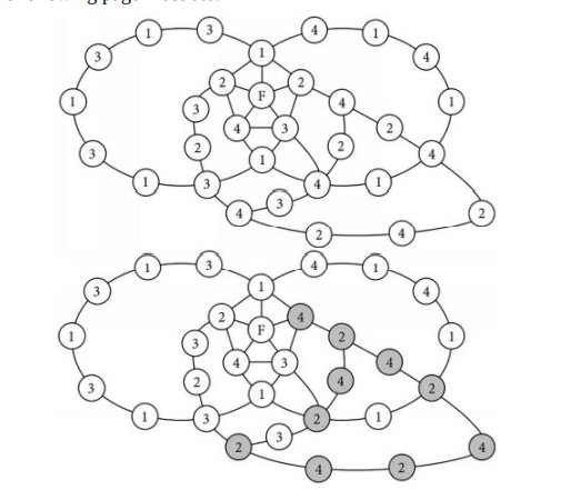
The graphs above are incomplete. These figures only show a vertex with degree four (vertex E), its nearest neighbors (A, B, C, and D), and segments of A-C Kempe chains. The entire graphs would also contain several other vertices (especially, more colored the same as B or D) and enough edges to be MPG’s. The left figure has A connected to $C$ in a single section of an A-C Kempe chain (meaning that the vertices of this chain are colored the same as A and C). The left figure shows that this A-C Kempe chain prevents B from connecting to $\mathrm{D}$ with a single section of a B-D Kempe chain. The middle figure has A and C in separate sections of A-C Kempe chains. In this case, B could connect to D with a single section of a B-D Kempe chain. However, since the A and C of the vertex with degree four lie on separate sections, the color of C’s chain can be reversed so that in the vertex with degree four, C is effectively recolored to match A’s color, as shown in the right figure. Similarly, D’s section could be reversed in the left figure so that D is effectively recolored to match B’s color.
Kempe also attempted to demonstrate that vertices with degree five are fourcolorable in his attempt to prove the four-color theorem [Ref. 2], but his argument for vertices with degree five was shown by Heawood in 1890 to be insufficient [Ref. 3]. Let’s explore what happens if we attempt to apply our reasoning for vertices with degree four to a vertex with degree five.
数学代写|图论作业代写Graph Theory代考|The previous diagrams
The previous diagrams show that when the two color reversals are performed one at a time in the crossed-chain graph, the first color reversal may break the other chain, allowing the second color reversal to affect the colors of one of F’s neighbors. When we performed the $2-4$ reversal to change B from 2 to 4 , this broke the 1-4 chain. When we then performed the 2-3 reversal to change E from 3, this caused C to change from 3 to 2 . As a result, F remains connected to four different colors; this wasn’t reversed to three as expected. Unfortunately, you can’t perform both reversals “at the same time” for the following reason. Let’s attempt to perform both reversals “at the same time.” In this crossed-chain diagram, when we swap 2 and 4 on B’s side of the 1-3 chain, one of the 4’s in the 1-4 chain may change into a 2, and when we swap 2 and 3 on E’s side of the 1-4 chain, one of the 3’s in the 1-3 chain may change into a 2 . This is shown in the following figure: one 2 in each chain is shaded gray. Recall that these figures are incomplete; they focus on one vertex (F), its neighbors (A thru E), and Kempe chains. Other vertices and edges are not shown.
Note how one of the 3’s changed into 2 on the left. This can happen when we reverse $\mathrm{C}$ and $\mathrm{E}$ (which were originally 3 and 2 ) on E’s side of the 1-4 chain. Note also how one of the 4’s changed into 2 on the right. This can happen when we reverse B and D (which were originally 2 and 4) outside of the 1-3 chain. Now we see where a problem can occur when attempting to swap the colors of two chains at the same time. If these two 2’s happen to be connected by an edge like the dashed edge shown above, if we perform the double reversal at the same time, this causes two vertices of the same color to share an edge, which isn’t allowed. We’ll revisit Kempe’s strategy for coloring a vertex with degree five in Chapter $25 .$
数学代写|图论作业代写Graph Theory代考| The shading of one section of the B-R
在上图中,顶点和是四度,因为它连接到其他四个顶点。Kempe 表明顶点 A、B、C 和 D 不能被强制为四种不同的颜色,这样顶点 E 总是可以被着色而不会违反四色定理,无论 MPG 的其余部分看起来如何上一页显示的部分。
A 和 C 或者是 AC Kempe 链的同一部分的一部分,或者它们各自位于 AC Kempe 链的不同部分。(如果一种和C例如,是红色和黄色的,则 AC 链是红黄色链。) – 如果一种和C每个位于 AC Kempe 链的不同部分,其中一个部分的颜色可以反转,这有效地重新着色 C 以匹配 A 的颜色。如果 A 和 C 是 AC Kempe 链的同一部分的一部分,则 B 和 D每个都必须位于 BD Kempe 链的不同部分,因为 AC Kempe 链将阻止任何 BD Kempe 链从 B 到达 D。(如果乙和D是蓝色和绿色,例如,那么一种BD Kempe 链是蓝绿色链。)在这种情况下,由于 B 和 D 分别位于 BD Kempe 链的不同部分,因此 BD Kempe 链的其中一个部分的颜色可以反转,这有效地重新着色 D 以匹配 B颜色。– 因此,可以使 C 与 A 具有相同的颜色或使 D 具有与 A 相同的颜色乙通过反转 Kempe 链的分离部分。
上面的图表是不完整的。这些图只显示了一个四阶顶点(顶点 E)、它的最近邻居(A、B、C 和 D),以及 AC Kempe 链的片段。整个图还将包含几个其他顶点(特别是与 B 或 D 相同的颜色)和足够多的边以成为 MPG。左图有 A 连接到C在 AC Kempe 链的单个部分中(意味着该链的顶点颜色与 A 和 C 相同)。左图显示此 AC Kempe 链阻止 B 连接到DBD Kempe 链条的一个部分。中间的数字在 AC Kempe 链的不同部分有 A 和 C。在这种情况下,B 可以通过 BD Kempe 链的单个部分连接到 D。但是,由于四阶顶点的 A 和 C 位于不同的部分,因此可以反转 C 链的颜色,以便在四阶顶点中,C 有效地重新着色以匹配 A 的颜色,如右图所示. 类似地,可以在左图中反转 D 的部分,以便有效地重新着色 D 以匹配 B 的颜色。
statistics-lab™ 为您的留学生涯保驾护航 在代写应用线性模型Applied Linear Models方面已经树立了自己的口碑, 保证靠谱, 高质且原创的统计Statistics代写服务。我们的专家在代写应用线性模型Applied Linear Models代写方面经验极为丰富,各种代写应用线性模型Applied Linear Models相关的作业也就用不着说。
我们提供的应用线性模型Applied Linear Models及其相关学科的代写,服务范围广, 其中包括但不限于:
Statistical Inference 统计推断
Statistical Computing 统计计算
Advanced Probability Theory 高等概率论
Advanced Mathematical Statistics 高等数理统计学
(Generalized) Linear Models 广义线性模型
Statistical Machine Learning 统计机器学习
Longitudinal Data Analysis 纵向数据分析
Foundations of Data Science 数据科学基础
统计代写|应用线性模型代写Applied Linear Models代考|STAT6420
统计代写|应用线性模型代写Applied Linear Models代考|Properties of solutions
One might now ask about the relationship, if any, between the two solutions (9) and (12) found by using the two generalized inverses $\mathbf{G}$ and $\dot{\mathbf{G}}$. Both satisfy (8) for an infinite number of sets of values of $z_3, z_4$ and $\dot{z}_1, \dot{z}_4$. The basic question is: Do the two solutions generate, through allocating different sets of values to the arbitrary values $z_3$ and $z_4$ in $\tilde{\mathbf{x}}$ and $\dot{z}_1$ and $\dot{z}_4$ in $\dot{\mathbf{x}}$, the same series of vectors that satisfy $\mathbf{A x}=\mathbf{y}$ ? The answer is “yes”. This is so because, on putting $\dot{z}_1=-6+z_3+29 z_4$ and $\dot{z}_4=z_4$, the solution in (12) becomes identical to that in (9). Hence (9) and (12) both generate the same sets of solutions to (8)
The relationship between solutions using $\mathbf{G}$ and those using $\dot{\mathbf{G}}$ is that, on putting $$ \tilde{\mathbf{x}} \text { reduces to } \dot{\mathbf{x}} \quad \mathbf{z}=(\mathbf{G}-\dot{\mathbf{G}}) \mathbf{y}+(\mathbf{I}-\dot{\mathbf{G} A}) \dot{\mathbf{z}}, $$ A stronger result, which concerns generation of all solutions from $\tilde{\mathbf{x}}$, is contained in the following theorem.
Theorem 3. For the consistent equations $\mathbf{A x}=\mathbf{y}$ all solutions are, for any specific G, generated by $\tilde{\mathbf{x}}=\mathbf{G y}+(\mathbf{G A}-\mathbf{I}) \mathbf{z}$, for arbitrary $\mathbf{z}$.
Proof. Let $\mathbf{x}^$ be any solution to $\mathbf{A x}=\mathbf{y}$. Choose $\mathbf{z}=(\mathbf{G A}-\mathbf{I}) \mathbf{x}^$ and it will be found that $\tilde{\mathbf{x}}$ reduces to $\mathbf{x}^*$. Thus, by appropriate choice of $\mathbf{z}$, any solution to $\mathbf{A x}=\mathbf{y}$ can be put in the form of $\tilde{\mathbf{x}}$.
The importance of this theorem is that one need derive only one generalized inverse of $\mathbf{A}$ in order to be able to generate all solutions to $\mathbf{A x}=\mathbf{y}$. There are no solutions other than those that can be generated from $\tilde{\mathbf{x}}$.
Having established a method for solving linear equations and shown that they can have an infinite number of solutions, we ask two questions: What relationships exist among the solutions and to what extent are the solutions linearly independent (LIN)? Since each solution is a vector of order $q$ there can, of course, be no more than $q$ LIN solutions. In fact there are fewer, as Theorem 4 shows. But first, a lemma.
统计代写|应用线性模型代写Applied Linear Models代考|OTHER DEFINITIONS
It is clear that the Penrose inverse $\mathbf{K}$ is not easy to compute, especially when $\mathbf{A}$ has many columns, because then the application of the Cayley-Hamilton theorem to $\mathbf{A}^{\prime} \mathbf{A}$ for obtaining $\mathbf{T}$ will be tedious. However, as has already been shown, only the first Penrose condition needs to be satisfied in order to have a matrix useful for solving linear equations. And in pursuing the topic of linear models it is found that this is the only condition really needed. It is for this reason that a generalized inverse of $\mathbf{A}$ has been defined as any matrix $\mathbf{G}$ that satisfies AGA = A, a definition that is retained throughout this book. Nevertheless, a variety of names are to be found in the literature, both for $\mathbf{G}$ and for other matrices satisfying fewer than all four of the Penrose conditions. A set of descriptive names is given in Table $1.1$.
In the notation of Table $1.1 \mathbf{A}^{(0)}=\mathbf{G}$, the generalized inverse already defined and discussed, and $\mathbf{A}^{(p)}=\mathbf{K}$, the Penrose inverse. This has also been called the pseudo inverse and the $p$-inverse by various authors. The suggested definition of a normalized generalized inverse in Table $1.1$ is not universally accepted. As given there, it is used by Urquhart (1968), whereas Goldman and Zelen (1964) call it a “weak” generalized inverse. An example of such a matrix is a left inverse $\mathbf{L}$ such that $\mathbf{L A}=\mathbf{I}$. The description “normalized” has also been used by Rohde (1966) for a matrix satisfying conditions (i), (ii) and (iv). An example of this kind of matrix is the right inverse $\mathbf{R}$ for which $\mathbf{A R}=\mathbf{I}$. Using the symbols of Table $1.1$ it can be seen that $$ \mathbf{A}^{(g)} \supset \mathbf{A}^{(r)} \supset \mathbf{A}^{(n)} \supset \mathbf{A}^{(p)} $$ namely that the set of matrices $\mathbf{A}^{(g)}$ includes all those that are reflexive, $\mathbf{A}^{(r)}$, which in turn includes all the normalized generalized inverses $\mathbf{A}^{(n)}$, which includes the unique $\mathbf{A}^{(p)}=\mathbf{K}$. Relationships between the four can be established as follows: $$ \begin{aligned} \mathbf{A}^{(r)} &=\mathbf{A}^{(g)} \mathbf{A} \mathbf{A}^{(g)} \ \mathbf{A}^{(n)} &=\mathbf{A}^{\prime}\left(\mathbf{A A}^{\prime}\right)^{(g)} \ \mathbf{A}^{(p)} &=\mathbf{A}^{\prime}\left(\mathbf{A A}^{\prime}\right)^{(g)} \mathbf{A}\left(\mathbf{A}^{\prime} \mathbf{A}\right)^{(g)} \mathbf{A}^{\prime} . \end{aligned} $$
The graphs above are incomplete. These figures only show a vertex with degree four (vertex E), its nearest neighbors (A, B, C, and D), and segments of A-C Kempe chains. The entire graphs would also contain several other vertices (especially, more colored the same as B or D) and enough edges to be MPG’s. The left figure has A connected to $C$ in a single section of an A-C Kempe chain (meaning that the vertices of this chain are colored the same as A and C). The left figure shows that this A-C Kempe chain prevents B from connecting to $\mathrm{D}$ with a single section of a B-D Kempe chain. The middle figure has A and C in separate sections of A-C Kempe chains. In this case, B could connect to D with a single section of a B-D Kempe chain. However, since the A and C of the vertex with degree four lie on separate sections, the color of C’s chain can be reversed so that in the vertex with degree four, C is effectively recolored to match A’s color, as shown in the right figure. Similarly, D’s section could be reversed in the left figure so that D is effectively recolored to match B’s color.
Kempe also attempted to demonstrate that vertices with degree five are fourcolorable in his attempt to prove the four-color theorem [Ref. 2], but his argument for vertices with degree five was shown by Heawood in 1890 to be insufficient [Ref. 3]. Let’s explore what happens if we attempt to apply our reasoning for vertices with degree four to a vertex with degree five.
数学代写|图论作业代写Graph Theory代考|The previous diagrams
The previous diagrams show that when the two color reversals are performed one at a time in the crossed-chain graph, the first color reversal may break the other chain, allowing the second color reversal to affect the colors of one of F’s neighbors. When we performed the $2-4$ reversal to change B from 2 to 4 , this broke the 1-4 chain. When we then performed the 2-3 reversal to change E from 3, this caused C to change from 3 to 2 . As a result, F remains connected to four different colors; this wasn’t reversed to three as expected. Unfortunately, you can’t perform both reversals “at the same time” for the following reason. Let’s attempt to perform both reversals “at the same time.” In this crossed-chain diagram, when we swap 2 and 4 on B’s side of the 1-3 chain, one of the 4’s in the 1-4 chain may change into a 2, and when we swap 2 and 3 on E’s side of the 1-4 chain, one of the 3’s in the 1-3 chain may change into a 2 . This is shown in the following figure: one 2 in each chain is shaded gray. Recall that these figures are incomplete; they focus on one vertex (F), its neighbors (A thru E), and Kempe chains. Other vertices and edges are not shown.
Note how one of the 3’s changed into 2 on the left. This can happen when we reverse $\mathrm{C}$ and $\mathrm{E}$ (which were originally 3 and 2 ) on E’s side of the 1-4 chain. Note also how one of the 4’s changed into 2 on the right. This can happen when we reverse B and D (which were originally 2 and 4) outside of the 1-3 chain. Now we see where a problem can occur when attempting to swap the colors of two chains at the same time. If these two 2’s happen to be connected by an edge like the dashed edge shown above, if we perform the double reversal at the same time, this causes two vertices of the same color to share an edge, which isn’t allowed. We’ll revisit Kempe’s strategy for coloring a vertex with degree five in Chapter $25 .$
数学代写|图论作业代写Graph Theory代考| The shading of one section of the B-R
在上图中,顶点和是四度,因为它连接到其他四个顶点。Kempe 表明顶点 A、B、C 和 D 不能被强制为四种不同的颜色,这样顶点 E 总是可以被着色而不会违反四色定理,无论 MPG 的其余部分看起来如何上一页显示的部分。
A 和 C 或者是 AC Kempe 链的同一部分的一部分,或者它们各自位于 AC Kempe 链的不同部分。(如果一种和C例如,是红色和黄色的,则 AC 链是红黄色链。) – 如果一种和C每个位于 AC Kempe 链的不同部分,其中一个部分的颜色可以反转,这有效地重新着色 C 以匹配 A 的颜色。如果 A 和 C 是 AC Kempe 链的同一部分的一部分,则 B 和 D每个都必须位于 BD Kempe 链的不同部分,因为 AC Kempe 链将阻止任何 BD Kempe 链从 B 到达 D。(如果乙和D是蓝色和绿色,例如,那么一种BD Kempe 链是蓝绿色链。)在这种情况下,由于 B 和 D 分别位于 BD Kempe 链的不同部分,因此 BD Kempe 链的其中一个部分的颜色可以反转,这有效地重新着色 D 以匹配 B颜色。– 因此,可以使 C 与 A 具有相同的颜色或使 D 具有与 A 相同的颜色乙通过反转 Kempe 链的分离部分。
上面的图表是不完整的。这些图只显示了一个四阶顶点(顶点 E)、它的最近邻居(A、B、C 和 D),以及 AC Kempe 链的片段。整个图还将包含几个其他顶点(特别是与 B 或 D 相同的颜色)和足够多的边以成为 MPG。左图有 A 连接到C在 AC Kempe 链的单个部分中(意味着该链的顶点颜色与 A 和 C 相同)。左图显示此 AC Kempe 链阻止 B 连接到DBD Kempe 链条的一个部分。中间的数字在 AC Kempe 链的不同部分有 A 和 C。在这种情况下,B 可以通过 BD Kempe 链的单个部分连接到 D。但是,由于四阶顶点的 A 和 C 位于不同的部分,因此可以反转 C 链的颜色,以便在四阶顶点中,C 有效地重新着色以匹配 A 的颜色,如右图所示. 类似地,可以在左图中反转 D 的部分,以便有效地重新着色 D 以匹配 B 的颜色。
statistics-lab™ 为您的留学生涯保驾护航 在代写应用线性模型Applied Linear Models方面已经树立了自己的口碑, 保证靠谱, 高质且原创的统计Statistics代写服务。我们的专家在代写应用线性模型Applied Linear Models代写方面经验极为丰富,各种代写应用线性模型Applied Linear Models相关的作业也就用不着说。
我们提供的应用线性模型Applied Linear Models及其相关学科的代写,服务范围广, 其中包括但不限于:
Statistical Inference 统计推断
Statistical Computing 统计计算
Advanced Probability Theory 高等概率论
Advanced Mathematical Statistics 高等数理统计学
(Generalized) Linear Models 广义线性模型
Statistical Machine Learning 统计机器学习
Longitudinal Data Analysis 纵向数据分析
Foundations of Data Science 数据科学基础
统计代写|应用线性模型代写Applied Linear Models代考|STAT3022
统计代写|应用线性模型代写Applied Linear Models代考|GENERALIZED INVERSE MATRICES
The application of generalized inverse matrices to linear statistical models is of relatively recent occurrence. As a mathematical tool such matrices aid in understanding certain aspects of the analysis procedures associated with linear models, especially the analysis of unbalanced data, a topic to which considerable attention is given in this book. An appropriate starting point is therefore a summary of the features of generalized inverse matrices that are important to linear models. Other ancillary results in matrix algebra are also discussed. a. Definition and existence A generalized inverse of a matrix $\mathbf{A}$ is defined, in this book, as any matrix $\mathbf{G}$ that satisfies the equation $$ \mathbf{A G A}=\mathbf{A} . $$ The name “generalized inverse” for matrices $\mathbf{G}$ defined by (1) is unfortunately not universally accepted, although it is used quite widely. Names such as “conditional inverse”, “pseudo inverse” and ” $g$-inverse” are also to be found in the literature, sometimes for matrices defined as is $\mathbf{G}$ of (1) and sometimes for matrices defined as variants of G. However, throughout this book the name “generalized inverse” of $\mathbf{A}$ is used exclusively for any matrix $\mathbf{G}$ satisfying (1).
Notice that (1) does not define $\mathbf{G}$ as “the” generalized inverse of $\mathbf{A}$ but as ” $a$ ” generalized inverse. This is because $\mathbf{G}$, for a given matrix $\mathbf{A}$, is not unique. As shown below, there is an infinite number of matrices $\mathbf{G}$ that satisfy (1) and so we refer to the whole class of them as generalized inverses of $\mathbf{A}$.
One way of illustrating the existence of $\mathbf{G}$ and its non-uniqueness starts with the equivalent diagonal form of $\mathbf{A}$. If $\mathbf{A}$ has order $p \times q$ the reduction to this diagonal form can be written as $$ \mathbf{P}{p \times p} \mathbf{A}{p \times q} \mathbf{Q}{q \times q}=\boldsymbol{\Delta}{p \times q} \equiv\left[\begin{array}{cl} \mathbf{D}{r \times r} & \mathbf{0}{r \times(q-r)} \ \mathbf{0}{(p-r) \times r} & \mathbf{0}{(p-r) \times(q-r)} \end{array}\right] $$ or, more simply, as $$ \mathbf{P A Q}=\Delta=\left[\begin{array}{cc} \mathbf{D}_r & 0 \ 0 & 0 \end{array}\right] . $$
统计代写|应用线性模型代写Applied Linear Models代考|Obtaining solutions
The link between a generalized inverse of the matrix $\mathbf{A}$ and consistent equations $\mathbf{A x}=\mathbf{y}$ is set out in the following theorem adapted from Rao (1962)
Theorem 1. Consistent equations $\mathbf{A x}=\mathbf{y}$ have a solution $\mathbf{x}=\mathbf{G y}$ if and only if $\mathbf{A G A}=\mathbf{A}$.
Proof. If the equations $\mathbf{A x}=\mathbf{y}$ are consistent and have $\mathbf{x}=\mathbf{G y}$ as a solution, write $\mathbf{a}_j$ for the $j$ th column of $\mathbf{A}$ and consider the equations $\mathbf{A x}=\mathbf{a}_j$. They have a solution: the null vector with its jth element set equal to unity. Therefore the equations $\mathbf{A x}=\mathbf{a}_j$ are consistent. Furthermore, since consistent equations $\mathbf{A x}=\mathbf{y}$ have a solution $\mathbf{x}=\mathbf{G y}$, it follows that consistent equations $\mathbf{A x}=\mathbf{a}_j$ have a solution $\mathbf{x}=\mathbf{G a}_j$. Therefore $\mathbf{A G a} \mathbf{a}_j=\mathbf{a}_j$; and this is true for all values of $j$, i.e., for all columns of $\mathbf{A}$. Hence $\mathbf{A G A}=\mathbf{A}$.
Conversely, if $\mathbf{A G A}=\mathbf{A}$, then $\mathbf{A G} \mathbf{A x}=\mathbf{A x}$, and when $\mathbf{A x}=\mathbf{y}$ this gives $\mathbf{A G y}=\mathbf{y}$, i.e., $\mathbf{A}(\mathbf{G} \mathbf{y})=\mathbf{y}$. Hence $\mathbf{x}=\mathbf{G y}$ is a solution of $\mathbf{A x}=\mathbf{y}$, and the theorem is proved.
Theorem 1 indicates how a solution to consistent equations may be obtained: find any matrix $\mathbf{G}$ satisfying $\mathbf{A G A}=\mathbf{A}$, i.e., find $\mathbf{G}$ as any generalized inverse of $\mathbf{A}$, and then $\mathbf{G y}$ is a solution. However, as Theorem 2 shows, Gy is not the only solution. There are, indeed, many solutions whenever $\mathbf{A}$ is anything other than a square, non-singular matrix.
Theorem 2. If $\mathbf{A}$ has $q$ columns and if $\mathbf{G}$ is a generalized inverse of $\mathbf{A}$, then the consistent equations $\mathbf{A x}=\mathbf{y}$ have solution $$ \tilde{\mathbf{x}}=\mathbf{G y}+(\mathbf{G A}-\mathbf{I}) \mathbf{z}, $$ where $\mathbf{z}$ is any arbitrary vector of order $q$. Proof. $\mathbf{A} \tilde{\mathbf{x}}=\mathbf{A G} \mathbf{y}+(\mathbf{A G A}-\mathbf{A}) \mathbf{z}$ $$ \begin{aligned} &=\mathbf{A G y}, \text { because } \mathbf{A} \mathbf{G A}=\mathbf{A}, \ &=\mathbf{y}, \text { by Theorem } 1 ; \end{aligned} $$ i.e., $\tilde{\mathbf{x}}$ satisfies $\mathbf{A x}=\mathbf{y}$ and hence is a solution. The notation $\tilde{\mathbf{x}}$ emphasizes that $\tilde{\mathbf{x}}$ is a solution, distinguishing it from the general vector of unknowns $\mathbf{x}$. Note that the solution $\tilde{\mathbf{x}}$ involves an element of arbitrariness because $\mathbf{z}$ is an arbitrary vector: $\mathbf{z}$ can have any value at all and $\tilde{\mathbf{x}}$ will still be a solution to $\mathbf{A x}=\mathbf{y}$. No matter what value is given to $\mathbf{z}$, the expression for $\tilde{\mathbf{x}}$ given in (7) satisfies $\mathbf{A x}=\mathbf{y}$. Furthermore, this will be so for whatever generalized inverse of $\mathbf{A}$ is used for $\mathbf{G}$
The graphs above are incomplete. These figures only show a vertex with degree four (vertex E), its nearest neighbors (A, B, C, and D), and segments of A-C Kempe chains. The entire graphs would also contain several other vertices (especially, more colored the same as B or D) and enough edges to be MPG’s. The left figure has A connected to $C$ in a single section of an A-C Kempe chain (meaning that the vertices of this chain are colored the same as A and C). The left figure shows that this A-C Kempe chain prevents B from connecting to $\mathrm{D}$ with a single section of a B-D Kempe chain. The middle figure has A and C in separate sections of A-C Kempe chains. In this case, B could connect to D with a single section of a B-D Kempe chain. However, since the A and C of the vertex with degree four lie on separate sections, the color of C’s chain can be reversed so that in the vertex with degree four, C is effectively recolored to match A’s color, as shown in the right figure. Similarly, D’s section could be reversed in the left figure so that D is effectively recolored to match B’s color.
Kempe also attempted to demonstrate that vertices with degree five are fourcolorable in his attempt to prove the four-color theorem [Ref. 2], but his argument for vertices with degree five was shown by Heawood in 1890 to be insufficient [Ref. 3]. Let’s explore what happens if we attempt to apply our reasoning for vertices with degree four to a vertex with degree five.
数学代写|图论作业代写Graph Theory代考|The previous diagrams
The previous diagrams show that when the two color reversals are performed one at a time in the crossed-chain graph, the first color reversal may break the other chain, allowing the second color reversal to affect the colors of one of F’s neighbors. When we performed the $2-4$ reversal to change B from 2 to 4 , this broke the 1-4 chain. When we then performed the 2-3 reversal to change E from 3, this caused C to change from 3 to 2 . As a result, F remains connected to four different colors; this wasn’t reversed to three as expected. Unfortunately, you can’t perform both reversals “at the same time” for the following reason. Let’s attempt to perform both reversals “at the same time.” In this crossed-chain diagram, when we swap 2 and 4 on B’s side of the 1-3 chain, one of the 4’s in the 1-4 chain may change into a 2, and when we swap 2 and 3 on E’s side of the 1-4 chain, one of the 3’s in the 1-3 chain may change into a 2 . This is shown in the following figure: one 2 in each chain is shaded gray. Recall that these figures are incomplete; they focus on one vertex (F), its neighbors (A thru E), and Kempe chains. Other vertices and edges are not shown.
Note how one of the 3’s changed into 2 on the left. This can happen when we reverse $\mathrm{C}$ and $\mathrm{E}$ (which were originally 3 and 2 ) on E’s side of the 1-4 chain. Note also how one of the 4’s changed into 2 on the right. This can happen when we reverse B and D (which were originally 2 and 4) outside of the 1-3 chain. Now we see where a problem can occur when attempting to swap the colors of two chains at the same time. If these two 2’s happen to be connected by an edge like the dashed edge shown above, if we perform the double reversal at the same time, this causes two vertices of the same color to share an edge, which isn’t allowed. We’ll revisit Kempe’s strategy for coloring a vertex with degree five in Chapter $25 .$
数学代写|图论作业代写Graph Theory代考| The shading of one section of the B-R
在上图中,顶点和是四度,因为它连接到其他四个顶点。Kempe 表明顶点 A、B、C 和 D 不能被强制为四种不同的颜色,这样顶点 E 总是可以被着色而不会违反四色定理,无论 MPG 的其余部分看起来如何上一页显示的部分。
A 和 C 或者是 AC Kempe 链的同一部分的一部分,或者它们各自位于 AC Kempe 链的不同部分。(如果一种和C例如,是红色和黄色的,则 AC 链是红黄色链。) – 如果一种和C每个位于 AC Kempe 链的不同部分,其中一个部分的颜色可以反转,这有效地重新着色 C 以匹配 A 的颜色。如果 A 和 C 是 AC Kempe 链的同一部分的一部分,则 B 和 D每个都必须位于 BD Kempe 链的不同部分,因为 AC Kempe 链将阻止任何 BD Kempe 链从 B 到达 D。(如果乙和D是蓝色和绿色,例如,那么一种BD Kempe 链是蓝绿色链。)在这种情况下,由于 B 和 D 分别位于 BD Kempe 链的不同部分,因此 BD Kempe 链的其中一个部分的颜色可以反转,这有效地重新着色 D 以匹配 B颜色。– 因此,可以使 C 与 A 具有相同的颜色或使 D 具有与 A 相同的颜色乙通过反转 Kempe 链的分离部分。
上面的图表是不完整的。这些图只显示了一个四阶顶点(顶点 E)、它的最近邻居(A、B、C 和 D),以及 AC Kempe 链的片段。整个图还将包含几个其他顶点(特别是与 B 或 D 相同的颜色)和足够多的边以成为 MPG。左图有 A 连接到C在 AC Kempe 链的单个部分中(意味着该链的顶点颜色与 A 和 C 相同)。左图显示此 AC Kempe 链阻止 B 连接到DBD Kempe 链条的一个部分。中间的数字在 AC Kempe 链的不同部分有 A 和 C。在这种情况下,B 可以通过 BD Kempe 链的单个部分连接到 D。但是,由于四阶顶点的 A 和 C 位于不同的部分,因此可以反转 C 链的颜色,以便在四阶顶点中,C 有效地重新着色以匹配 A 的颜色,如右图所示. 类似地,可以在左图中反转 D 的部分,以便有效地重新着色 D 以匹配 B 的颜色。