ACTL20001 - 统计代写答疑辅导

标签： ACTL20001

金融代写|金融数学代写Financial Mathematics代考|ACTL20001

Posted on 2022年9月21日2022年9月21日 by statistics-lab

如果你也在怎样代写金融数学Financial Mathematics这个学科遇到相关的难题，请随时右上角联系我们的24/7代写客服。

金融数学是将数学方法应用于金融问题。(有时使用的同等名称是定量金融、金融工程、数学金融和计算金融）。它借鉴了概率、统计、随机过程和经济理论的工具。传统上，投资银行、商业银行、对冲基金、保险公司、公司财务部和监管机构将金融数学的方法应用于诸如衍生证券估值、投资组合结构、风险管理和情景模拟等问题。依赖商品的行业（如能源、制造业）也使用金融数学。定量分析为金融市场和投资过程带来了效率和严谨性，在监管方面也变得越来越重要。

statistics-lab™ 为您的留学生涯保驾护航在代写金融数学Financial Mathematics方面已经树立了自己的口碑, 保证靠谱, 高质且原创的统计Statistics代写服务。我们的专家在代写金融数学Financial Mathematics代写方面经验极为丰富，各种代写金融数学Financial Mathematics相关的作业也就用不着说。

我们提供的金融数学Financial Mathematics及其相关学科的代写，服务范围广, 其中包括但不限于:

Statistical Inference 统计推断
Statistical Computing 统计计算
Advanced Probability Theory 高等概率论
Advanced Mathematical Statistics 高等数理统计学
(Generalized) Linear Models 广义线性模型
Statistical Machine Learning 统计机器学习
Longitudinal Data Analysis 纵向数据分析
Foundations of Data Science 数据科学基础

金融代写|金融数学代写Financial Mathematics代考|ACTL20001

金融代写|金融数学代写Financial Mathematics代考|Option Combination Strategies

Option combinations involve simultaneous positions in at least one call option and at least one put option. This section focuses on combinations of calls and puts with the same expiration date and underlying asset. The synthetic long positions in the underlying asset using options (long a call and short a put) and short positions (long a put and short a call) discussed in Section $1.8 .1$ are option combinations. This section discusses others.

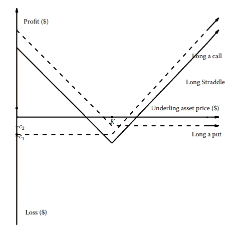
Option straddles have equally sized simultaneous long positions or simultaneous short positions in call and put options with the same strike price (and same expiration date). Figure $1.12$ illustrates the profitability of a long straddle at expiration with a solid line and shows the underlying components of long a call and long a put with dashed lines. The value of a long straddle is positively exposed to the volatility of the underlying asset. A short straddle is the mirror image (i.e., the maximum profit is above $K$ with losses on the far right and left).

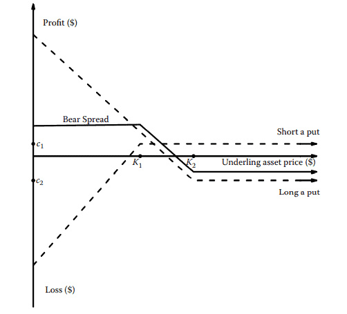
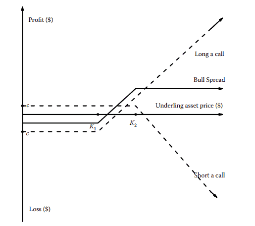
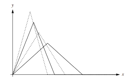
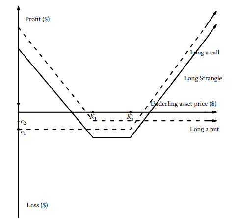
Option strangles are similar to option straddles, except the call and put options have different strike prices. Figure $1.13$ illustrates a long strangle. Other options strategies can involve option portfolios such as ratio spreads with more calls than puts or vice versa such that the payoffs differ in different directions.

金融代写|金融数学代写Financial Mathematics代考|Other Options

There are many types of stand-alone options on financial assets that differ from simple calls and puts. Some options allow exercise at several specific points in time (a Bermuda option), some are based on functions of prices such as averages or extremes (e.g., Asian options have payoffs based on averaged prices of the underlying asset). Some options cease to exist if the underlying asset reaches a particular level or become exercisable if the underlying asset reaches a particular level such as barrier options.
Financial markets and economic activity in general are full of options. There are options on real assets such as options to: buy land, rent space, return products, extend warrantees, take early retirement, terminate contracts, and on and on.

There are non-traded financial options such as options to pre-pay mortgages and other loans, options to break some bank certificates of deposits (i.e., receive early termination), options to rollover some bank deposits, options to cash out insurance policies, options to increase insurance coverage, and so forth.

The common stock of a leveraged corporation can be viewed as a call option on the corporation’s stock. There are even options on options known as compound options.
Two things to keep in mind are this: (1) there are countless implicit and explicit options in a modern economy because those options serve important purposes of allowing participants to manage and control their risk exposures and (2) the astounding variety and complexity of these important contracts creates demand for people with mathematical modeling skills, especially those who can create innovations or at least understand and model the innovations. This book touches on the most common options in existence today. No one can yet imagine the options that will emerge in the future to meet the changing needs of our rapidly changing world.

金融数学代考

金融代写|金融数学代写金融数学代考|选项组合策略

. .

期权组合包括至少一个看涨期权和至少一个看跌期权的同时头寸。本节重点介绍具有相同到期日和标的资产的看涨期权和看跌期权的组合。使用期权在标的资产中合成的多头头寸(做多看涨期权和做空看跌期权)和做空头寸(做多看跌期权和做空看涨期权)在$1.8 .1$节中讨论的是期权组合。

期权跨空具有相同执行价格(和相同到期日)的看涨期权和看跌期权的同时多头头寸或同时空头头寸。图$1.12$用实线说明了到期时多头跨空期权的盈利能力，用虚线显示了多头看涨期权和多头看跌期权的基本组成部分。多头多头的价值受到标的资产波动的正面影响。空头跨空是镜像(即最大利润在$K$以上，亏损在最右和最左)

除了看涨期权和看跌期权的执行价格不同之外，期权绞杀期权与期权跨空期权类似。图$1.13$说明了一个长时间的扼杀。其他期权策略可以包括期权组合，如看涨期权多于看跌期权，反之亦然，从而使不同方向的收益不同

金融代写|金融数学代写金融数学代考|其他选项

金融资产的独立期权有许多类型，不同于简单的看涨期权和看跌期权。有些期权允许在几个特定的时间点执行(百慕大期权)，有些则基于价格的函数，如平均值或极值(例如，亚洲期权的支付基于标的资产的平均价格)。如果标的资产达到特定水平，则有些期权将不复存在;如果标的资产达到特定水平，则有些期权将变为可执行期权，如障碍期权。金融市场和经济活动总体上充满了选择。在实物资产上有多种选择，如购买土地、租赁空间、返还产品、延长保修期、提前退休、终止合同等等

有一些非交易金融期权，如提前支付抵押贷款和其他贷款的期权，打破一些银行存款凭证的期权(即，接受提前终止)，展期一些银行存款的期权，套现保险单的期权，增加保险承保范围的期权，等等

杠杆公司的普通股可以被看作是公司股票的看涨期权。甚至还有被称为复合期权的期权。需要记住的两件事是:(1)在现代经济中有无数的隐性和显性选项，因为这些选项的重要目的是让参与者管理和控制他们的风险敞口;(2)这些重要契约的惊人多样性和复杂性创造了对具有数学建模技能的人的需求，特别是那些能够创造创新或至少理解和建模创新的人。这本书涉及到当今最常见的选择。没有人能想象未来会出现什么样的选择来满足我们这个迅速变化的世界不断变化的需求.

金融代写|金融数学代写Financial Mathematics代考请认准statistics-lab™

统计代写请认准statistics-lab™. statistics-lab™为您的留学生涯保驾护航。

金融工程代写

金融工程是使用数学技术来解决金融问题。金融工程使用计算机科学、统计学、经济学和应用数学领域的工具和知识来解决当前的金融问题，以及设计新的和创新的金融产品。

非参数统计代写

非参数统计指的是一种统计方法，其中不假设数据来自于由少数参数决定的规定模型；这种模型的例子包括正态分布模型和线性回归模型。

广义线性模型代考

广义线性模型（GLM）归属统计学领域，是一种应用灵活的线性回归模型。该模型允许因变量的偏差分布有除了正态分布之外的其它分布。

术语广义线性模型（GLM）通常是指给定连续和/或分类预测因素的连续响应变量的常规线性回归模型。它包括多元线性回归，以及方差分析和方差分析（仅含固定效应）。

有限元方法代写

有限元方法（FEM）是一种流行的方法，用于数值解决工程和数学建模中出现的微分方程。典型的问题领域包括结构分析、传热、流体流动、质量运输和电磁势等传统领域。

有限元是一种通用的数值方法，用于解决两个或三个空间变量的偏微分方程（即一些边界值问题）。为了解决一个问题，有限元将一个大系统细分为更小、更简单的部分，称为有限元。这是通过在空间维度上的特定空间离散化来实现的，它是通过构建对象的网格来实现的：用于求解的数值域，它有有限数量的点。边界值问题的有限元方法表述最终导致一个代数方程组。该方法在域上对未知函数进行逼近。[1] 然后将模拟这些有限元的简单方程组合成一个更大的方程系统，以模拟整个问题。然后，有限元通过变化微积分使相关的误差函数最小化来逼近一个解决方案。

tatistics-lab作为专业的留学生服务机构，多年来已为美国、英国、加拿大、澳洲等留学热门地的学生提供专业的学术服务，包括但不限于Essay代写，Assignment代写，Dissertation代写，Report代写，小组作业代写，Proposal代写，Paper代写，Presentation代写，计算机作业代写，论文修改和润色，网课代做，exam代考等等。写作范围涵盖高中，本科，研究生等海外留学全阶段，辐射金融，经济学，会计学，审计学，管理学等全球99%专业科目。写作团队既有专业英语母语作者，也有海外名校硕博留学生，每位写作老师都拥有过硬的语言能力，专业的学科背景和学术写作经验。我们承诺100%原创，100%专业，100%准时，100%满意。

随机分析代写

随机微积分是数学的一个分支，对随机过程进行操作。它允许为随机过程的积分定义一个关于随机过程的一致的积分理论。这个领域是由日本数学家伊藤清在第二次世界大战期间创建并开始的。

时间序列分析代写

随机过程，是依赖于参数的一组随机变量的全体，参数通常是时间。随机变量是随机现象的数量表现，其时间序列是一组按照时间发生先后顺序进行排列的数据点序列。通常一组时间序列的时间间隔为一恒定值（如1秒，5分钟，12小时，7天，1年），因此时间序列可以作为离散时间数据进行分析处理。研究时间序列数据的意义在于现实中，往往需要研究某个事物其随时间发展变化的规律。这就需要通过研究该事物过去发展的历史记录，以得到其自身发展的规律。

回归分析代写

多元回归分析渐进（Multiple Regression Analysis Asymptotics）属于计量经济学领域，主要是一种数学上的统计分析方法，可以分析复杂情况下各影响因素的数学关系，在自然科学、社会和经济学等多个领域内应用广泛。

MATLAB代写

MATLAB 是一种用于技术计算的高性能语言。它将计算、可视化和编程集成在一个易于使用的环境中，其中问题和解决方案以熟悉的数学符号表示。典型用途包括：数学和计算算法开发建模、仿真和原型制作数据分析、探索和可视化科学和工程图形应用程序开发，包括图形用户界面构建MATLAB 是一个交互式系统，其基本数据元素是一个不需要维度的数组。这使您可以解决许多技术计算问题，尤其是那些具有矩阵和向量公式的问题，而只需用 C 或 Fortran 等标量非交互式语言编写程序所需的时间的一小部分。MATLAB 名称代表矩阵实验室。MATLAB 最初的编写目的是提供对由 LINPACK 和 EISPACK 项目开发的矩阵软件的轻松访问，这两个项目共同代表了矩阵计算软件的最新技术。MATLAB 经过多年的发展，得到了许多用户的投入。在大学环境中，它是数学、工程和科学入门和高级课程的标准教学工具。在工业领域，MATLAB 是高效研究、开发和分析的首选工具。MATLAB 具有一系列称为工具箱的特定于应用程序的解决方案。对于大多数 MATLAB 用户来说非常重要，工具箱允许您学习和应用专业技术。工具箱是 MATLAB 函数（M 文件）的综合集合，可扩展 MATLAB 环境以解决特定类别的问题。可用工具箱的领域包括信号处理、控制系统、神经网络、模糊逻辑、小波、仿真等。

R语言代写	问卷设计与分析代写
PYTHON代写	回归分析与线性模型代写
MATLAB代写	方差分析与试验设计代写
STATA代写	机器学习/统计学习代写
SPSS代写	计量经济学代写
EVIEWS代写	时间序列分析代写
EXCEL代写	深度学习代写
SQL代写	各种数据建模与可视化代写

金融代写|金融数学代写Financial Mathematics代考|Find2022

Posted on 2022年9月21日2022年9月21日 by statistics-lab

如果你也在怎样代写金融数学Financial Mathematics这个学科遇到相关的难题，请随时右上角联系我们的24/7代写客服。

我们提供的金融数学Financial Mathematics及其相关学科的代写，服务范围广, 其中包括但不限于:

Statistical Inference 统计推断
Statistical Computing 统计计算
Advanced Probability Theory 高等概率论
Advanced Mathematical Statistics 高等数理统计学
(Generalized) Linear Models 广义线性模型
Statistical Machine Learning 统计机器学习
Longitudinal Data Analysis 纵向数据分析
Foundations of Data Science 数据科学基础

金融代写|金融数学代写Financial Mathematics代考|Find2022

金融代写|金融数学代写Financial Mathematics代考|Arbitrage-Free Binomial Option Valuation

One of the most fascinating models of arbitrage-free derivative valuation is a binomial option pricing model. A binomial model allows only two possible outcomes to the value of a share of stock over a single time period. Each possible outcome is termed a “state,” which is often described as being an “up state” or a “down state.”
For example, consider a share of stock currently trading at $\$ 10$ per share that is viewed as having two possible outcomes at the end of one year: $\$ 16$ if things go well (the up state) and $\$ 7$ is things go poorly (the down state). We denote the current price of the stock as $S_0$, the value of the stock price in the up state as $S_u$ and the value of the stock in the down state as $S_d$. This simplest of all binomial models is illustrated in Figure $1.6$ for a single time period.Now consider a call option on that stock that expires in one period and has a strike price of $\$ 13$. While we do not yet know the market value of that option, $C_0$, we do know that the value of the option at the end of the year ( $C_u$ in the up state and $C_d$ in the down state) from the payoffs of $\$ 3$ in the up state (found as $\$ 16-\$ 13$ ) and $\$ 0$ in the down state (because the option is not exercised) as depicted in Figure 1.7.

Note that the stock price varies by $\$ 9$ between the two states (i.e., $\$ 16-\$ 7$ ) at the same time that the option price varies by only $\$ 3$. The key to solving for the current option price $\left(C_0\right)$ begins by realizing that the payoffs to the option are perfectly correlated with the payoffs to the stock. The only differences are that the stock price varies three times as much and the stock price has a worst case value of $\$ 7$ while the option has a worst-case value of $\$ 0$. This means that an arbitrager can construct two portfolios with identical payoffs, which is called replicating one portfolio using the other. Here, two portfolios are constructed: (1) one or more call options plus one riskless bond and (2) one share of the stock. The two portfolios are constructed to have the same payoffs at the option’s expiration. If their payoffs are identical, then their current values must be identical. To replicate the stock using a call option and a bond, the payoffs must be the same. The first step is to note that if the options expire worthlessly the riskless bond must have the same payoff as the stock in the down state (in this case $\$ 7)$. Therefore, the riskless bond must have a face value of $\$ 7$. The second step is to determine the number of call options which, combined with the bond, will offer the same payout at the option’s expiration as the stock in the upstate (\$16). The number of call options, $h$, must be such that:
Payoff in upstate $=\$ 16=$ bond $+(h \times$ call $)=\$ 7+(h \times \$ 3)$
$$
h=(\$ 16-\$ 7) / \$ 3=3
$$

金融代写|金融数学代写Financial Mathematics代考|Popular Option Strategies with Multiple Positions

Two of the most popular strategies involving options are covered calls and protective puts. Both of these strategies were illustrated in the examples in Section 1.5.1. A covered call is the simultaneous writing of a call option while having a long position in the underlying asset. A protective put is the simultaneous purchase of a put option while having a long position in the underlying asset. These two portfolios are depicted in Figure $1.8$ and Figure $1.9$

Note that the portfolio profits and losses in Figures $1.8$ and $1.9$ can be formed by summing the profits and losses of the portfolio’s component positions. In other words, at each point on the horizontal axis (i.e., each value of $S_T$ ), the profit or loss of the covered call or protective put is found by summing the profits and/or losses of the two positions that form them.

Option spreads are simultaneous long and short positions in either different call options or different put options (but not both calls and puts). Three general types of option spread strategies are vertical spreads, horizontal spreads, and diagonal spreads. The terms describing the three spreads relate to the visualization of a matrix of option prices with strike price forming the vertical axis and expiration date forming the horizontal axis. Thus, in a vertical option spread, the options differ by strike price; in a horizontal option spread, the options differ by expiration date; and in a diagonal spread, they differ by both strike price and expiration date. This section focuses on the strategies with the same expiration date – vertical spreads.

Figure $1.10$ illustrates a vertical call spread known as a bull spread. The payout of a bull spread at expiration is positively related to the underlying asset, hence it is “bullish” with respect to the price of the underlying asset. The bullish nature of a bull spread occurs when the long call option position is in the option with the lower strike price and the short option position is in the asset with the higher strike price. Interestingly, the same bullish diagram can be generated using put options with the same structure: the long put option position is in the option with the lower strike price and the short option position is in the asset with the higher strike price.

Figure $1.11$ illustrates a vertical call spread known as a bear spread. Bear spreads reverse the direction of the options by establishing the long call option position in the option with the higher strike price and the short option position is in the asset with the lower strike price. Like in the case of bull spreads, the same bearish diagram can be generated using put options with the same structure: the long put option position is in the option with the higher strike price and the short option position is in the asset with the lower strike price.

金融数学代考

金融代写|金融数学代写金融数学代考|无套利二项期权估值

无套利衍生品估值最吸引人的模型之一是二项期权定价模型。二项模型只允许一股股票在一段时间内的价值产生两种可能的结果。每种可能的结果都被称为“状态”，通常被描述为“向上状态”或“向下状态”。例如，考虑一股目前交易价格为每股$\$ 10$的股票，它被认为在一年底有两种可能的结果:如果情况顺利(上升状态)，它的价格为$\$ 16$;如果情况不顺利(下降状态)，它的价格为$\$ 7$。我们将股票的当前价格表示为$S_0$，将处于上涨状态的股价值表示为$S_u$，将处于下跌状态的股票值表示为$S_d$。图$1.6$说明了所有二项模型中最简单的一个时间段。现在考虑这只股票的看涨期权，在一个时期内到期，执行价为$\$ 13$。虽然我们还不知道该期权的市场价值$C_0$，但我们确实知道该期权在年底的价值($C_u$在上升状态，$C_d$在下降状态)从$\$ 3$在上升状态(发现为$\$ 16-\$ 13$)和$\$ 0$在下降状态(因为该期权没有被执行)的支付，如图1.7所示

注意，股票价格在两种状态(即$\$ 16-\$ 7$)之间的变化是$\$ 9$，而与此同时，期权价格只变化$\$ 3$。解决当前期权价格$\left(C_0\right)$的关键是要意识到期权的收益与股票的收益是完全相关的。唯一的区别是股价的变化是三倍，股价的最坏情况值是$\$ 7$，而期权的最坏情况值是$\$ 0$。这意味着一个套利者可以构建两个具有相同收益的投资组合，这被称为用一个投资组合复制另一个投资组合。这里，我们构建了两个投资组合:(1)一个或多个看涨期权加上一个无风险债券和(2)一股股票。这两种投资组合在期权到期时的收益是相同的。如果它们的收益相同，那么它们的现值也一定相同。用看涨期权和债券来复制股票，收益必须是相同的。第一步是要注意，如果期权到期时毫无价值，无风险债券的支付必须与下跌状态下的股票相同(在这种情况下是$\$ 7)$)。因此，无风险债券的面值必须为$\$ 7$。第二步是确定看涨期权的数量，这些看涨期权与债券相结合，在期权到期时提供的股息与北部州的股票(16美元)相同。看涨期权的数量$h$必须满足以下条件:
在上州的偿付$=\$ 16=$ bond $+(h \times$ call $)=\$ 7+(h \times \$ 3)$
$$
h=(\$ 16-\$ 7) / \$ 3=3
$$

金融代写|金融数学代写金融数学代考|多仓位热门期权策略

涉及期权的两种最流行的策略是备兑看涨期权和保护性看跌期权。这两种策略都在1.5.1节的例子中进行了说明。备兑买入是指在持有标的资产多头头寸的同时，同时卖出看涨期权。保护性看跌期权是在持有标的资产多头头寸的同时买入看跌期权。这两个投资组合在图$1.8$和图$1.9$ 中描述

注意，图$1.8$和$1.9$中的投资组合损益可以由投资组合中各组成头寸的损益相加而成。换句话说，在横轴上的每一点(即$S_T$的每一个值)，补兑看涨期权或保护性看跌期权的盈亏是通过将构成补兑看涨期权或保护性看跌期权的两个头寸的盈亏相加得到的

期权价差是同时持有不同看涨期权或看跌期权的多头和空头头寸(但不是同时持有看涨和看跌期权)。期权价差策略有三种:垂直价差、水平价差和对角线价差。描述这三种价差的术语与期权价格矩阵的可视化有关，执行价格构成纵轴，到期日期构成横轴。因此，在垂直期权价差中，期权的执行价格不同;在水平期权价差中，期权的到期日不同;在对角线价差中，执行价格和到期日都不同。本节主要讨论具有相同到期日的策略——垂直价差

图$1.10$显示了被称为牛市价差的垂直呼叫价差。到期时多头价差的支付与标的资产正相关，因此相对于标的资产的价格，它是“看涨”的。当看涨期权的多头头寸是执行价较低的期权，而空头头寸是执行价较高的资产时，看涨价差的看涨性质就发生了。有趣的是，使用具有相同结构的看跌期权也可以生成相同的看涨图:多头看跌期权头寸位于执行价较低的期权中，而空头期权头寸位于执行价较高的资产中

图$1.11$显示了被称为空头价差的垂直买入价差。空头价差扭转了期权的走势，在执行价较高的期权上建立看涨期权多头头寸，在执行价较低的资产上建立空头头寸。就像在牛市价差的情况下，使用具有相同结构的看跌期权可以生成相同的看跌图:多头看跌期权头寸位于执行价较高的期权中，而空头期权头寸位于执行价较低的资产中

统计代写请认准statistics-lab™. statistics-lab™为您的留学生涯保驾护航。

金融工程代写

非参数统计代写

非参数统计指的是一种统计方法，其中不假设数据来自于由少数参数决定的规定模型；这种模型的例子包括正态分布模型和线性回归模型。

广义线性模型代考

广义线性模型（GLM）归属统计学领域，是一种应用灵活的线性回归模型。该模型允许因变量的偏差分布有除了正态分布之外的其它分布。

有限元方法代写

随机分析代写

时间序列分析代写

回归分析代写

MATLAB代写

R语言代写	问卷设计与分析代写
PYTHON代写	回归分析与线性模型代写
MATLAB代写	方差分析与试验设计代写
STATA代写	机器学习/统计学习代写
SPSS代写	计量经济学代写
EVIEWS代写	时间序列分析代写
EXCEL代写	深度学习代写
SQL代写	各种数据建模与可视化代写

金融代写|金融数学代写Financial Mathematics代考|ACFl1003

Posted on 2022年7月21日2022年7月21日 by statistics-lab

如果你也在怎样代写金融数学Financial Mathematics这个学科遇到相关的难题，请随时右上角联系我们的24/7代写客服。

我们提供的金融数学Financial Mathematics及其相关学科的代写，服务范围广, 其中包括但不限于:

Statistical Inference 统计推断
Statistical Computing 统计计算
Advanced Probability Theory 高等概率论
Advanced Mathematical Statistics 高等数理统计学
(Generalized) Linear Models 广义线性模型
Statistical Machine Learning 统计机器学习
Longitudinal Data Analysis 纵向数据分析
Foundations of Data Science 数据科学基础

金融代写|金融数学代写Financial Mathematics代考|ACFl1003

金融代写|金融数学代写Financial Mathematics代考|Sequences of functions

Given a real interval $[a, b]$, we denote $\mathscr{F}([a, b])$ the collection of all real functions defined on $[a, b]$ :
$$
\mathscr{F}([a, b])={f \mid f:[a, b] \rightarrow \mathbb{R}} .
$$
Definition 2.2. A sequence of functions with domain $[a, b]$ is a sequence of elements of $\mathscr{F}([a, b])$.

Example 2.3. Functions $f_{n}(x)=x^{n}$, where $x \in[0,1]$, form a sequence of functions in $\mathscr{F}([0,1])$.

Let us analyse what happens when $n \rightarrow \infty$. It is easy to realise that a sequence of continuous functions may converge to a non-continuous function. Indeed, for the sequence of functions in Example 2.3, it holds:
$$
\lim {n \rightarrow \infty} f{n}(x)=\lim {n \rightarrow \infty} x^{n}= \begin{cases}1 & \text { if } \quad x=1 \ 0 & \text { if } \quad 0 \leq x<1\end{cases} $$ Thus, even if every function of the sequence $f{n}(x)=x^{n}$ is continuous, the limit function $f(x)$, defined below, may not be continuous:
$$
f(x):=\lim {n \rightarrow \infty} f{n}(x) .
$$
The convergence of a sequence of functions, like that of Example 2.3, is called simple convergence. We now provide its rigorous definition.

金融代写|金融数学代写Financial Mathematics代考|Uniform convergence

Pointwise convergence does not allow, in general, interchanging between limit and integral operators, a possibility that we call passage to the limit and that we also address in $\S$ 8.10. To explain it, consider the sequence of functions:
$$
f_{n}(x)=n e^{-n^{2} x^{2}}
$$
defined on $[0, \infty)$; it is a sequence that clearly converges to the zero function. Employing the substitution $n x=y$, evaluation of the integral of $f_{n}$ yields:
$$
\int_{0}^{\infty} f_{n}(x) \mathrm{d} x=\int_{0}^{\infty} e^{-y^{2}} \mathrm{~d} y
$$
We do not have the tools, yet, to evaluate the integral in the left-hand side of the above equality (but we will soon), but it is clear that it is a positive real number, so we have:
$$
\lim {n \rightarrow \infty} \int{0}^{\infty} f_{n}(x) \mathrm{d} x=\int_{0}^{\infty} e^{-y^{2}} \mathrm{~d} y=\alpha>0 \neq \int_{0}^{\infty} \lim {n \rightarrow \infty} f{n}(x) \mathrm{d} x=0 .
$$
To establish a ‘good’ notion of convergence, that allows the passage to the limit, when we take the integral of the considered sequence, and that preserves continuity, we introduce the fundamental notion of uniform convergence.

金融数学代考

金融代写|金融数学代写Financial Mathematics代考|Sequences of functions

给定一个真实的区间 $[a, b]$ ，我们表示 $\mathscr{F}([a, b])$ 上定义的所有实函数的集合 $[a, b]$ :
$$
\mathscr{F}([a, b])=f \mid f:[a, b] \rightarrow \mathbb{R} .
$$
定义 2.2。具有域的函数序列 $[a, b]$ 是一系列元素 $\mathscr{F}([a, b])$.
例 2.3。功能 $f_{n}(x)=x^{n}$ ，在哪里 $x \in[0,1]$ ，形成一个函数序列 $\mathscr{F}([0,1])$.
让我们分析一下当 $n \rightarrow \infty$. 很容易意识到一系列连续函数可能会收敛到一个非连续函数。实际上，对于示例 $2.3$ 中的函数序列，它成立:
$$
\lim n \rightarrow \infty f n(x)=\lim n \rightarrow \infty x^{n}={1 \quad \text { if } \quad x=10 \quad \text { if } \quad 0 \leq x<1
$$
因此，即使序列的每个函数 $f n(x)=x^{n}$ 是连续的，极限函数 $f(x)$ ，定义如下，可能不是连续的:
$$
f(x):=\lim n \rightarrow \infty f n(x) .
$$
一系列函数的收敛，如例 $2.3$ 中的收敛，称为简单收敛。我们现在提供它的严格定义。

金融代写|金融数学代写Financial Mathematics代考|Uniform convergence

逐点收敛通常不允许极限和积分算子之间的交换，我们称之为通过极限的可能性，我们也在 $8.10$ 。为了解释它，考虑函数的顺序:
$$
f_{n}(x)=n e^{-n^{2} x^{2}}
$$
定义于 $[0, \infty)$; 这是一个明显收敛到零函数的序列。使用替代品 $n x=y$, 积分的评价 $f_{n}$ 产量:
$$
\int_{0}^{\infty} f_{n}(x) \mathrm{d} x=\int_{0}^{\infty} e^{-y^{2}} \mathrm{~d} y
$$
我们还没有工具来评估上述等式左侧的积分（但我们很快就会这样做），但很明显它是一个正实数，所以我们有:
$$
\lim n \rightarrow \infty \int 0^{\infty} f_{n}(x) \mathrm{d} x=\int_{0}^{\infty} e^{-y^{2}} \mathrm{~d} y=\alpha>0 \neq \int_{0}^{\infty} \lim n \rightarrow \infty f n(x) \mathrm{d} x=0
$$
为了建立一个”好的”收敛概念，允许通过极限，当我们对所考虑的序列进行积分并保持连续性时，我们引入了一致收敛的基本概念。

统计代写请认准statistics-lab™. statistics-lab™为您的留学生涯保驾护航。

金融工程代写

非参数统计代写

非参数统计指的是一种统计方法，其中不假设数据来自于由少数参数决定的规定模型；这种模型的例子包括正态分布模型和线性回归模型。

广义线性模型代考

广义线性模型（GLM）归属统计学领域，是一种应用灵活的线性回归模型。该模型允许因变量的偏差分布有除了正态分布之外的其它分布。

有限元方法代写

随机分析代写

时间序列分析代写

回归分析代写

MATLAB代写

R语言代写	问卷设计与分析代写
PYTHON代写	回归分析与线性模型代写
MATLAB代写	方差分析与试验设计代写
STATA代写	机器学习/统计学习代写
SPSS代写	计量经济学代写
EVIEWS代写	时间序列分析代写
EXCEL代写	深度学习代写
SQL代写	各种数据建模与可视化代写

金融代写|金融数学代写Financial Mathematics代考|MATH3090

Posted on 2022年7月21日2022年7月21日 by statistics-lab

如果你也在怎样代写金融数学Financial Mathematics这个学科遇到相关的难题，请随时右上角联系我们的24/7代写客服。

我们提供的金融数学Financial Mathematics及其相关学科的代写，服务范围广, 其中包括但不限于:

Statistical Inference 统计推断
Statistical Computing 统计计算
Advanced Probability Theory 高等概率论
Advanced Mathematical Statistics 高等数理统计学
(Generalized) Linear Models 广义线性模型
Statistical Machine Learning 统计机器学习
Longitudinal Data Analysis 纵向数据分析
Foundations of Data Science 数据科学基础

金融代写|金融数学代写Financial Mathematics代考|MATH3090

金融代写|金融数学代写Financial Mathematics代考|Limits of functions

A vector function is a function $f$ of the form $f: A \rightarrow \mathbb{R}^{m}$, where $A \subset \mathbb{R}^{n}$. Since $f(\boldsymbol{x}) \in \mathbb{R}^{m}$ for each $\boldsymbol{x} \in A$, then there are $m$ functions $f_{j}: A \rightarrow \mathbb{R}$, calléd component functions ớ $f$, such that:
$$
f(\boldsymbol{x})=\left(f_{1}(\boldsymbol{x}), \ldots, f_{m}(\boldsymbol{x})\right) \quad \text { for each } \quad \boldsymbol{x} \in A
$$
When $m=1$, function $f$ has only one component and we call $f$ real-valued. If $f=\left(f_{1}, \ldots, f_{m}\right)$ is a vector function, where the components $f_{j}$ have intrinsic domains, then the maximal domain of $f$ is defined to be the intersection of the domains of all components $f_{j}$.

To set up a notation for the algebra of vector functions, let $E \subset \mathbb{R}^{n}$ and let $f, g: E \rightarrow \mathbb{R}^{m}$. For each $x \in E$, the following operations can be defined.
The scalar multiple of $\alpha \in \mathbb{R}$ by $f$ is given by:
$$
(\alpha f)(\boldsymbol{x}):=\alpha f(\boldsymbol{x}) .
$$
The sum of $f$ and $g$ is obtained as:
$$
(f+g)(\boldsymbol{x}):=f(\boldsymbol{x})+g(\boldsymbol{x}) .
$$
The (Euclidean) dot product of $f$ and $g$ is constructed as:
$$
(f \cdot g)(\boldsymbol{x}):=f(\boldsymbol{x}) \cdot g(\boldsymbol{x}) .
$$

金融代写|金融数学代写Financial Mathematics代考|Sequences and series of real or complex numbers

A sequence is a set of numbers $u_{1}, u_{2}, u_{3}, \ldots$, in a definite order of arrangement, that is, a map $u: \mathbb{N} \rightarrow \mathbb{R}$ or $u: \mathbb{N} \rightarrow \mathbb{C}$, formed according to a certain rule. Each number in the sequence is called term; $u_{n}$ is called the $n^{\text {th }}$ term. The sequence is called finite or infinite, according to the number of terms. The sequence $u_{1}, u_{2}, u_{3}, \ldots$, when considered as a function, is also designated as $\left(u_{n}\right){n \in \mathbb{N}}$ or briefly $\left(u{n}\right)$.

Definition 2.1. The real or complex number $\ell$ is called the limit of the infinite sequence $\left(u_{n}\right)$ if, for any positive number $\varepsilon$, there exists a positive number $n_{\varepsilon}$, depending on $\varepsilon$, such that $\left|u_{n}-\ell\right|<\varepsilon$ for all integers $n>n_{\varepsilon}$. In such a case, we denote:
$$
\lim {n \rightarrow \infty} u{n}=\ell
$$
Given a sequence $\left(u_{n}\right)$, we say that its associated infinite series $\sum_{n=1}^{\infty} u_{n}$ :
(i) converges, when it exists the limit:
$$
\lim {n \rightarrow \infty} \sum{k=1}^{n} u_{k}:=S=\sum_{n=1}^{\infty} u_{n}
$$
(ii) diverges, when the limit of the partial sums $\sum_{k=1}^{n} u_{k}$ does not exist.

金融数学代考

金融代写|金融数学代写Financial Mathematics代考|Limits of functions

向量函数是一个函数 $f$ 形式的 $f: A \rightarrow \mathbb{R}^{m}$ ，在哪里 $A \subset \mathbb{R}^{n}$. 自从 $f(\boldsymbol{x}) \in \mathbb{R}^{m}$ 对于每个 $\boldsymbol{x} \in A$, 那么有 $m$ 功能 $f_{j}: A \rightarrow \mathbb{R}$ ，称为组件函数 ớ $f$ ，这样:
$$
f(\boldsymbol{x})=\left(f_{1}(\boldsymbol{x}), \ldots, f_{m}(\boldsymbol{x})\right) \quad \text { for each } \quad \boldsymbol{x} \in A
$$
什么时候 $m=1$ ，功能 $f$ 只有一个组件，我们称之为 $f$ 实值。如果 $f=\left(f_{1}, \ldots, f_{m}\right)$ 是一个向量函数，其中分量 $f_{j}$ 有内在域，那么最大域 $f$ 被定义为所有组件域的交集 $f_{j}$.
要为向量函数的代数建立一个符号，让 $E \subset \mathbb{R}^{n}$ 然后让 $f, g: E \rightarrow \mathbb{R}^{m}$. 对于每个 $x \in E$ ，可以定义以下操作。的标量倍数 $\alpha \in \mathbb{R}$ 经过 $f$ 是 (谁) 给的:
$$
(\alpha f)(\boldsymbol{x}):=\alpha f(\boldsymbol{x})
$$
总数是 $f$ 和 $g$ 获得为:
$$
(f+g)(\boldsymbol{x}):=f(\boldsymbol{x})+g(\boldsymbol{x}) .
$$
的 (欧几里得) 点积 $f$ 和 $g$ 构造为:
$$
(f \cdot g)(\boldsymbol{x}):=f(\boldsymbol{x}) \cdot g(\boldsymbol{x})
$$

金融代写|金融数学代写Financial Mathematics代考|Sequences and series of real or complex numbers

序列是一组数字 $u_{1}, u_{2}, u_{3}, \ldots$ ，按一定的排列顺序，也就是一张图 $u: \mathbb{N} \rightarrow \mathbb{R}$ 或者 $u: \mathbb{N} \rightarrow \mathbb{C}$ ，按照一定的规律形成。序列中的每个数字称为项; $u_{n}$ 被称为 $n^{\text {th }}$ 学期。根据项的数量，该序列称为有限或无限。序列 $u_{1}, u_{2}, u_{3}, \ldots$ ，当被视为一个函数时，也被指定为 $\left(u_{n}\right) n \in \mathbb{N}$ 或简要 $(u n)$.
定义 2.1。实数或复数 $\ell$ 称为无限序列的极限 $\left(u_{n}\right)$ 如果，对于任何正数 $\varepsilon$ ，存在一个正数 $n_{\varepsilon}$ ，根据 $\varepsilon$ ，这样 $\left|u_{n}-\ell\right|<\varepsilon$ 对于所有整数 $n>n_{\varepsilon}$. 在这种情况下，我们表示:
$$
\lim n \rightarrow \infty u n=\ell
$$
给定一个序列 $\left(u_{n}\right)$ ，我们说它相关的无穷级数 $\sum_{n=1}^{\infty} u_{n}$ :
(i) 收敛，当它存在极限时:
$$
\lim n \rightarrow \infty \sum k=1^{n} u_{k}:=S=\sum_{n=1}^{\infty} u_{n}
$$
(ii) 发散，当部分和的限制 $\sum_{k=1}^{n} u_{k}$ 不存在。

统计代写请认准statistics-lab™. statistics-lab™为您的留学生涯保驾护航。

金融工程代写

非参数统计代写

非参数统计指的是一种统计方法，其中不假设数据来自于由少数参数决定的规定模型；这种模型的例子包括正态分布模型和线性回归模型。

广义线性模型代考

广义线性模型（GLM）归属统计学领域，是一种应用灵活的线性回归模型。该模型允许因变量的偏差分布有除了正态分布之外的其它分布。

有限元方法代写

随机分析代写

时间序列分析代写

回归分析代写

MATLAB代写

R语言代写	问卷设计与分析代写
PYTHON代写	回归分析与线性模型代写
MATLAB代写	方差分析与试验设计代写
STATA代写	机器学习/统计学习代写
SPSS代写	计量经济学代写
EVIEWS代写	时间序列分析代写
EXCEL代写	深度学习代写
SQL代写	各种数据建模与可视化代写

金融代写|金融数学代写Financial Mathematics代考|ACTL20001

Posted on 2022年7月21日2022年7月21日 by statistics-lab

如果你也在怎样代写金融数学Financial Mathematics这个学科遇到相关的难题，请随时右上角联系我们的24/7代写客服。

我们提供的金融数学Financial Mathematics及其相关学科的代写，服务范围广, 其中包括但不限于:

Statistical Inference 统计推断
Statistical Computing 统计计算
Advanced Probability Theory 高等概率论
Advanced Mathematical Statistics 高等数理统计学
(Generalized) Linear Models 广义线性模型
Statistical Machine Learning 统计机器学习
Longitudinal Data Analysis 纵向数据分析
Foundations of Data Science 数据科学基础

金融代写|金融数学代写Financial Mathematics代考|Euclidean space

If $n \in \mathbb{N}$, we use the symbol $\mathbb{R}^{n}$ to indicate the Cartesian ${ }^{1}$ product of $n$ copies of $\mathbb{R}$ with itself, i.e.:
$$
\mathbb{R}^{n}:=\left{\left(x_{1}, x_{2}, \ldots, x_{n}\right) \mid x_{j} \in \mathbb{R} \text { for } j=1,2, \ldots, n\right} .
$$
The concept of Euclidean ${ }^{2}$ space is not limited to the set $\mathbb{R}^{n}$, but it also includes the so-called Euclidean inner product, introduced in Definition 1.1. The integer $n$ is called dimension of $\mathbb{R}^{n}$, the elements $x=\left(x_{1}, x_{2}, \ldots, x_{n}\right)$ of $\mathbb{R}^{n}$ are called points, or vectors or ordered $n$-tuples, while $x_{j}, j=1, \ldots, n$, are the coordinates, or components, of $\boldsymbol{x}$. Vectors $\boldsymbol{x}$ and $\boldsymbol{y}$ are equal if $x_{j}=y_{j}$ for $j=1,2, \ldots, n$. The zero vector is the vector whose components are null, that is, $\mathbf{0}:=(0,0, \ldots, 0)$. In low dimension situations, i.e. for $n=2$ or $n=3$, we will write $\boldsymbol{x}=(x, y)$ and $\boldsymbol{x}=(x, y, z)$, respectively.

For our purposes, that is extending differential calculus to functions of several variables, we need to define an algebraic structure in $\mathbb{R}^{n}$. This is done by introducing operations in $\mathbb{R}^{n}$.

Definition 1.1. Let $\boldsymbol{x}=\left(x_{1}, x_{2}, \ldots, x_{n}\right), \boldsymbol{y}=\left(y_{1}, y_{2}, \ldots, y_{n}\right) \in \mathbb{R}^{n}$ and $\alpha \in \mathbb{R}$
(i) The sum of $\boldsymbol{x}$ and $\boldsymbol{y}$ is the vector:
$$
\boldsymbol{x}+\boldsymbol{y}:=\left(x_{1}+y_{1}, x_{2}+y_{2}, \ldots, x_{n}+y_{n}\right) ;
$$

(ii) The difference of $\boldsymbol{x}$ and $\boldsymbol{y}$ is the vector:
$$
\boldsymbol{x}-\boldsymbol{y}:=\left(x_{1}-y_{1}, x_{2}-y_{2}, \ldots, x_{n}-y_{n}\right)
$$
(iii) The $\alpha$-multiple of $\boldsymbol{x}$ is the vector:
$$
\alpha \boldsymbol{x}=\left(\alpha x_{1}, \alpha x_{2}, \ldots, \alpha x_{n}\right) ;
$$
(iv) The Euclidean inner product of $\boldsymbol{x}$ and $\boldsymbol{y}$ is the real number:
$$
\boldsymbol{x} \cdot \boldsymbol{y}:=x_{1} y_{1}+x_{2} y_{2}+\ldots+x_{n} y_{n} .
$$

金融代写|金融数学代写Financial Mathematics代考|Topology of R

Topology, that is the description of the relations among subsets of $\mathbb{R}^{n}$, is based on the concept of open and closed sets, that generalises the notion of open and closed intervals. After introducing these concepts, we state their most basic properties. The first step is the natural generalisation of intervals in $\mathbb{R}^{n}$

Definition 1.13. Open and closed balls are defined as follows:
(i) $\forall r>0$, the open ball, centered at $a$, of radius $r$, is the set of points:
$$
B_{r}(\boldsymbol{a}):=\left{\boldsymbol{x} \in \mathbb{R}^{n} \mid|\boldsymbol{x}-\boldsymbol{a}|<r\right} ;
$$
(ii) $\forall r \geq 0$, the closed ball, centered at $\boldsymbol{a}$, of radius $r$, is the set of points:
$$
\bar{B}_{r}(\boldsymbol{a})\left{\boldsymbol{x} \in \mathbb{R}^{n}|| \mid \boldsymbol{x}-\boldsymbol{a} | \leq r\right}
$$
Note that, when $n=1$, the open ball centered at $a$ of radius $r$ is the open interval $(a-r, a+r)$, and the corresponding closed ball is the closed interval $[a-r, a+r]$. Here we adopt the convention of representing open balls as dashed circumferences, while closed balls are drawn as solid circumferences, as shown in Figure $1.4 .$

金融数学代考

金融代写|金融数学代写Financial Mathematics代考|Euclidean space

如果 $n \in \mathbb{N}$ ，我们使用符号 $\mathbb{R}^{n}$ 表示笛卡尔 ${ }^{1}$ 的产品 $n$ 的副本 $\mathbb{R}$ 本身，即:
$\backslash$ Imathbb ${R} \wedge{n}:=\backslash$ left $\left{\backslash\right.$ left $\left(x_{-}{1}, x_{-}{2}, \backslash\right.$ dots, $x_{-}{n} \backslash$ right) $\backslash$ mid $\left.\left.x_{-}\right} j\right}$ in $\backslash$ mathbb ${R} \backslash$ text ${$ for $} j=1,2, \backslash$ dots, $n \backslash$ right $}$ 。
欧几里得的概念 ${ }^{2}$ 空间不限于集合 $\mathbb{R}^{n}$ ，但它也包括定义 $1.1$ 中介绍的所谓欧几里得内积。整数 $n$ 被称为维度 $\mathbb{R}^{n}$ ，要素 $x=\left(x_{1}, x_{2}, \ldots, x_{n}\right)$ 的 $\mathbb{R}^{n}$ 被称为点、向量或有序 $n$-元组，而 $x_{j}, j=1, \ldots, n$, 是坐标或分量 $\boldsymbol{x}$. 矢量图 $\boldsymbol{x}$ 和 $\boldsymbol{y}$ 相等，如果 $x_{j}=y_{j}$ 为了 $j=1,2, \ldots, n$. 零向量是其分量为空的向量，即 $0:=(0,0, \ldots, 0)$. 在低维情况下，即对于 $n=2$ 或者 $n=3$ ，我们会写 $\boldsymbol{x}=(x, y)$ 和 $\boldsymbol{x}=(x, y, z)$ ，分别。
为了我们的目的，即将溦积分扩展到多个变量的函数，我们需要定义一个代数结构 $\mathbb{R}^{n}$. 这是通过在 $\mathbb{R}^{n}$.
定义 1.1。让 $\boldsymbol{x}=\left(x_{1}, x_{2}, \ldots, x_{n}\right), \boldsymbol{y}=\left(y_{1}, y_{2}, \ldots, y_{n}\right) \in \mathbb{R}^{n}$ 和 $\alpha \in \mathbb{R}$
$(-)$ 总和 $\boldsymbol{x}$ 和 $\boldsymbol{y}$ 是向量:
$$
\boldsymbol{x}+\boldsymbol{y}:=\left(x_{1}+y_{1}, x_{2}+y_{2}, \ldots, x_{n}+y_{n}\right)
$$
(ii) 差异 $\boldsymbol{x}$ 和 $\boldsymbol{y}$ 是向量:
$$
\boldsymbol{x}-\boldsymbol{y}:=\left(x_{1}-y_{1}, x_{2}-y_{2}, \ldots, x_{n}-y_{n}\right)
$$
(iii) $\alpha$ – 倍数 $\boldsymbol{x}$ 是向量:
$$
\alpha \boldsymbol{x}=\left(\alpha x_{1}, \alpha x_{2}, \ldots, \alpha x_{n}\right)
$$
(iv) 的欧几里得内积 $\boldsymbol{x}$ 和 $\boldsymbol{y}$ 是实数:
$$
\boldsymbol{x} \cdot \boldsymbol{y}:=x_{1} y_{1}+x_{2} y_{2}+\ldots+x_{n} y_{n}
$$

金融代写|金融数学代写Financial Mathematics代考|Topology of R

拓扑，即描述子集之间的关系 $\mathbb{R}^{n}$ ，基于开集和闭集的概念，它概括了开区间和闭区间的概念。在介绍了这些概念之后，我们陈述它们最基本的属性。第一步是区间的自然泛化 $\mathbb{R}^{n}$
定义 1.13。开球和闭球的定义如下:
(i) $\forall r>0$ ，开球, 以 $a$, 半径 $r$ ，是点的集合:
(二) $\forall r \geq 0$, 封闭球, 以 $\boldsymbol{a}$, 半径 $r$, 是点的集合:
请注意，当 $n=1$ ，空位球的中心在 $a$ 半径 $r$ 是开区间 $(a-r, a+r)$ ，对应的闭球就是闭区间 $[a-r, a+r]$. 这里我们采用将开球表示为虚线圆周的惯例，而将闭球表示为实心圆周，如图所示 $1.4 .$

统计代写请认准statistics-lab™. statistics-lab™为您的留学生涯保驾护航。

金融工程代写

非参数统计代写

非参数统计指的是一种统计方法，其中不假设数据来自于由少数参数决定的规定模型；这种模型的例子包括正态分布模型和线性回归模型。

广义线性模型代考

广义线性模型（GLM）归属统计学领域，是一种应用灵活的线性回归模型。该模型允许因变量的偏差分布有除了正态分布之外的其它分布。

有限元方法代写

随机分析代写

时间序列分析代写

回归分析代写

MATLAB代写

R语言代写	问卷设计与分析代写
PYTHON代写	回归分析与线性模型代写
MATLAB代写	方差分析与试验设计代写
STATA代写	机器学习/统计学习代写
SPSS代写	计量经济学代写
EVIEWS代写	时间序列分析代写
EXCEL代写	深度学习代写
SQL代写	各种数据建模与可视化代写

金融代写|金融数学代写Financial Mathematics代考|MATH3090

Posted on 2022年7月2日2022年7月2日 by statistics-lab

如果你也在怎样代写金融数学Financial Mathematics这个学科遇到相关的难题，请随时右上角联系我们的24/7代写客服。

我们提供的金融数学Financial Mathematics及其相关学科的代写，服务范围广, 其中包括但不限于:

Statistical Inference 统计推断
Statistical Computing 统计计算
Advanced Probability Theory 高等概率论
Advanced Mathematical Statistics 高等数理统计学
(Generalized) Linear Models 广义线性模型
Statistical Machine Learning 统计机器学习
Longitudinal Data Analysis 纵向数据分析
Foundations of Data Science 数据科学基础

金融代写|金融数学代写Financial Mathematics代考|Market Prices, Risk, and Randomness

Risk is a fascinating topic that is central to financial economics. What causes risk, and what causes security prices to change? The answers to these questions and the study of financial risk in general have progressed primarily using financial math.

The terms value and price (as well as the terms valuation and pricing) are often used interchangeably in finance. This book tends to use the term value to describe how much a particular person believes an item is worth and uses the term price to describe the amount of money that people receive or pay when they exchange the item. However, the term asset pricing is used frequently in financial economics to describe very important models even when the context is more clearly described as involving asset valuation.

Since the general meaning of the terms are quite similar, this book often uses the terms price and pricing to describe values and valuation in cases where price and pricing are conventionally used.

The value of an asset tends to change through time because the preferences of people change through time and the abilities of a modern economy to meet those preferences changes through time. Agricultural prices change due to factors such as weather, energy prices change due to factors such as economic activity, and stock prices change due to factors such as predictions of future revenues and expenses. Prices respond to changes as soon as the information about those changes is revealed. The effects of a frost on orange harvests begin changing market prices of orange juice when the weather is forecasted, not just when the damage is done.

The spot price is the price today for delivery today. The spot price of an asset such as a stock or bond reflects a consensus in the marketplace with regard to the future benefits that the asset offers. As time passes, the asset price changes because the market’s predictions of future conditions change. More generally, asset prices change because of the arrival of new information. Good news for a stock such as higher forecasts of earnings causes a positive price change, while bad news such as a disappointment regarding the sales of a new product causes a negative price change. To the extent that market participants rationally and efficiently process available information to form the current price of an asset, it follows that future price changes will be based on the arrival of new information.

Therefore, security prices can be viewed as random variables that change through time based on the arrival of new information. Simply put, the future price of an asset can be modeled as being equal to its future expected value plus or minus price changes due to new information that becomes available to market participants.

金融代写|金融数学代写Financial Mathematics代考|Expected Value as a Foundation of Asset Valuation

The starting point for valuing a financial asset is that the price of the asset should reflect the expected cash inflows that the asset offers. We know that future cash flows are uncertain. In order to find expected cash flows, we have to use probability models to model the likelihood of cash flows occurring. Let’s review some mathematics with a focus on expected value.

Expected value’s intuitive meaning is that it is a long-run average. If a random variable is sampled many times, the long-run average of these sampled values is the expected value of the variable. We begin by reviewing how to calculate expected value from probability model perspective.

In a competitive market, a financial asset’s price is determined by supply and demand. To simplify an example, let’s consider an asset that will distribute its final cash flow to the owner of the asset immediately (e.g., before the end of the day). Financial analysts compete to identify and purchase assets with current market prices below the asset’s expected distribution (i.e., final payoff) and to identify and sell assets with current market prices above their expected payoff. Thus the expected value of the random payoff of a financial asset drives the current market price of the asset. Throughout this book, we assume that financial analysts have estimates of the probability distribution of these random variables (i.e., asset or security prices). Without going into detail here about how the values of expected cash flows are adjusted for time (i.e., for the delay between buying an asset and receiving its payoffs) and risk (i.e., the uncertainty of the size and timing of future payoffs), the value of a financial asset or contract is based on expected cash flows as indicated in Basic Principle 1.1.

Let’s look at some simple examples of assets or contracts with random future payoffs and calculate their expected values. To simplify the first example, future cash flows are not discounted for time or risk. Later examples in this chapter include discounting for time and risk.

金融数学代考

金融代写|金融数学代写Financial Mathematics代考|Market Prices, Risk, and Randomness

风险是一个引人入胜的话题，是金融经济学的核心。是什么导致了风险，又是什么导致了证券价格的变化？这些问题的答案和一般金融风险的研究主要使用金融数学取得了进展。

术语价值和价格（以及术语估值和定价）在金融中经常互换使用。这本书倾向于使用价值这个词来描述一个特定的人认为一件物品的价值，并使用价格这个词来描述人们在交换物品时收到或支付的金额。然而，资产定价一词在金融经济学中经常用于描述非常重要的模型，即使上下文被更清楚地描述为涉及资产估值。

由于这些术语的一般含义非常相似，因此本书经常使用术语价格和定价来描述通常使用价格和定价的情况下的价值和估值。

资产的价值往往会随着时间而变化，因为人们的偏好会随着时间而变化，而现代经济满足这些偏好的能力也会随着时间而变化。农产品价格因天气等因素而变化，能源价格因经济活动等因素而变化，股票价格因未来收入和支出预测等因素而变化。一旦有关这些变化的信息被披露，价格就会对变化做出反应。霜冻对橙子收成的影响在预测天气时开始改变橙汁的市场价格，而不仅仅是在损害发生时。

现货价格是今天交割的价格。股票或债券等资产的现货价格反映了市场对资产提供的未来收益的共识。随着时间的推移，资产价格会发生变化，因为市场对未来状况的预测会发生变化。更一般地说，资产价格会随着新信息的到来而发生变化。对股票的好消息（例如更高的收益预测）会导致价格上涨，而坏消息（例如对新产品销售的失望）会导致价格下跌。如果市场参与者合理有效地处理可用信息以形成资产的当前价格，那么未来的价格变化将基于新信息的到来。

因此，证券价格可以被视为随机变量，随着新信息的到来而随时间变化。简而言之，资产的未来价格可以建模为等于其未来预期价值加上或减去市场参与者可获得的新信息导致的价格变化。

金融代写|金融数学代写Financial Mathematics代考|Expected Value as a Foundation of Asset Valuation

评估金融资产的出发点是资产价格应反映资产提供的预期现金流入。我们知道未来的现金流是不确定的。为了找到预期现金流，我们必须使用概率模型来模拟现金流发生的可能性。让我们回顾一些关注期望值的数学。

期望值的直观含义是它是一个长期平均值。如果一个随机变量被多次采样，这些采样值的长期平均值就是该变量的期望值。我们首先回顾如何从概率模型的角度计算期望值。

在竞争激烈的市场中，金融资产的价格是由供求关系决定的。为简化示例，让我们考虑一种资产，它将立即（例如，在一天结束之前）将其最终现金流分配给资产所有者。金融分析师竞相识别和购买当前市场价格低于资产预期分配（即最终收益）的资产，并竞争识别和出售当前市场价格高于其预期收益的资产。因此，金融资产随机收益的预期值推动了资产的当前市场价格。在本书中，我们假设金融分析师已经估计了这些随机变量（即资产或证券价格）的概率分布。此处不详细说明预期现金流的值如何随时间调整（即。

让我们看一些具有随机未来收益的资产或合约的简单示例，并计算它们的期望值。为了简化第一个例子，未来现金流量没有因时间或风险而贴现。本章后面的例子包括时间和风险贴现。

统计代写请认准statistics-lab™. statistics-lab™为您的留学生涯保驾护航。

金融工程代写

非参数统计代写

非参数统计指的是一种统计方法，其中不假设数据来自于由少数参数决定的规定模型；这种模型的例子包括正态分布模型和线性回归模型。

广义线性模型代考

广义线性模型（GLM）归属统计学领域，是一种应用灵活的线性回归模型。该模型允许因变量的偏差分布有除了正态分布之外的其它分布。

有限元方法代写

随机分析代写

时间序列分析代写

回归分析代写

MATLAB代写

R语言代写	问卷设计与分析代写
PYTHON代写	回归分析与线性模型代写
MATLAB代写	方差分析与试验设计代写
STATA代写	机器学习/统计学习代写
SPSS代写	计量经济学代写
EVIEWS代写	时间序列分析代写
EXCEL代写	深度学习代写
SQL代写	各种数据建模与可视化代写

金融代写|金融数学代写Financial Mathematics代考|ACTL20001

Posted on 2022年7月2日2022年7月2日 by statistics-lab

如果你也在怎样代写金融数学Financial Mathematics这个学科遇到相关的难题，请随时右上角联系我们的24/7代写客服。

我们提供的金融数学Financial Mathematics及其相关学科的代写，服务范围广, 其中包括但不限于:

Statistical Inference 统计推断
Statistical Computing 统计计算
Advanced Probability Theory 高等概率论
Advanced Mathematical Statistics 高等数理统计学
(Generalized) Linear Models 广义线性模型
Statistical Machine Learning 统计机器学习
Longitudinal Data Analysis 纵向数据分析
Foundations of Data Science 数据科学基础

金融代写|金融数学代写Financial Mathematics代考|The Roles of Financial Mathematics and Financial Derivatives

Financial mathematics has provided powerful tools for the development, understanding, and use of the wide spectrum of innovative financial products that have exploded in availability since the 1970 s. These financial products have tremendously expanded our abilities to exchange, manage, control, and understand economic risk. Economic risk is intangible and tends to be difficult to understand. Yet it is clear that those economies that develop the greatest skills and tools for dealing with economic risk are best able to harness the incredible power of economic trade and growth to meet the needs and wants of a large society. Financial mathematics lies at the heart of that past success and our ability to create future opportunities.
For example, a large operating firm such as an airline company faces a number of huge economic uncertainties regarding their revenues and expenses. What effects will fuel costs, labor costs, and financing costs have on their profitability and, ultimately, the firm’s ability to continue to provide transportation services? What factors will determine the revenues for forthcoming quarters and years? Will exchange rates and airplane prices change in directions that will prevent the airline company from purchasing new equipment to replace aging aircraft or to open new routes?

Financial derivatives can help the airline company control for risks external to the firm such as changing energy costs, interest rates, and exchange rates. By offsetting or hedging the effects of these otherwise uncontrollable external variables, the company can focus their attention on dealing with those matters over which they have dircct control: operating their firm with efficiency, safety, and high-quality service.

Financial derivatives have also played roles in creating or exacerbating financial crises at the international, individual investor, and firm levels. Clearly, derivatives are powerful tools that when used improperly can be as damaging as they are beneficial when used properly.

The key to effective management of financial risk is effective valuation. In finance, valuation of assets in general and financial derivatives in particular involves valuing prospective cash flows based on the timing of those cash flows and their risk. A good definition of finance is that it is the economics of time and risk. This chapter begins with highly simplified examples that ignore the effects of the timing of cash flows and the risk of cash flows on current values. Then the analyses will be expanded to include the time value of money (using forward contracts as an example) and the potential effects of risk on asset values (using options as an example).

金融代写|金融数学代写Financial Mathematics代考|The Roles of Arbitragers, Hedgers, and Speculators

Hull (2015) discusses three types of traders: ${ }^{1}$ arbitragers, hedgers, and speculators. Arbitragers, hedgers, and speculators, along with investors, borrowers, and entrepreneurs, all commonly use markets for financial securities and financial derivatives. Understanding the roles of arbitragers, hedgers, and speculators is helpful in understanding why derivatives have emerged and evolved into diverse forms.

An important concept before discussing these roles is short selling. The idea that a trader can take a short position in a financial derivative was introduced. It makes sense that, as a contract between two people regarding the price of an asset one of the parties to the contract will take the long side and one will take the short side. Having the long side of the contract means that one will have the risk exposure more similar to owning the asset with the other side having an exposure similar to owing the asset. Short selling is the process of obtaining the opposite exposure of owing an asset by borrowing the asset and selling it into the market at the current market price. The short seller of an asset therefore is inversely exposed to the price changes of the underlying asset: the short seller gains if the underlying stock or other asset’s market price falls and loses market value if the asset rises in value. Eventually, the short seller purchases the asset and returns it to the entity from which it was borrowed, terminating the short sale. Ignoring dividends and the time value of money, the short seller of a stock gains $\$ X$ if the stock declines $\$ X$ over the life of the short sale and loses $\$ X$ if the stock rises by $\$ X$.

Arbitragers are traders who establish a long (or buy) position in one or more assets that they believe are relatively underpriced and one or more short (or sell) positions in assets that they believe are relatively overpriced. Arbitragers hold these positions based on their belief that the prices will revert to more proper price levels that allow the arbitrager to exit hoth positions at a net profit. When markets are poorly or inefficiently priced, arbitragers can earn riskless or virtually riskless profits. Successful arbitragers serve the market by correcting pricing errors thereby (and unintentionally) ensuring that less informed market participants are transacting at prices that are nearer to their proper or equilibrium values. The distinguishing feature of arbitragers is that their trades are designed to take very little risk and tend to be short term.

金融数学代考

金融代写|金融数学代写Financial Mathematics代考|The Roles of Financial Mathematics and Financial Derivatives

金融数学为开发、理解和使用自 1970 年代以来广泛使用的创新金融产品提供了强大的工具。这些金融产品极大地扩展了我们交换、管理、控制和理解经济风险的能力。经济风险是无形的，往往难以理解。然而，很明显，那些发展出最强大的技能和工具来应对经济风险的经济体最能利用经济贸易和增长的强大力量来满足大社会的需求。金融数学是过去成功的核心，也是我们创造未来机会的能力的核心。
例如，航空公司等大型运营公司在收入和支出方面面临许多巨大的经济不确定性。燃料成本、劳动力成本和融资成本对其盈利能力以及最终对公司继续提供运输服务的能力有何影响？哪些因素将决定未来季度和年度的收入？汇率和飞机价格的变化是否会阻止航空公司购买新设备来更换老化的飞机或开辟新航线？

金融衍生品可以帮助航空公司控制公司外部的风险，例如不断变化的能源成本、利率和汇率。通过抵消或对冲这些无法控制的外部变量的影响，公司可以将注意力集中在处理他们直接控制的问题上：以高效、安全和高质量的服务运营公司。

金融衍生品也在国际、个人投资者和公司层面造成或加剧金融危机方面发挥了作用。显然，衍生工具是强大的工具，如果使用不当，它们的破坏性可能与正确使用时的益处一样大。

有效管理财务风险的关键是有效估值。在金融领域，一般资产和金融衍生品的估值涉及根据这些现金流的时间及其风险对预期现金流进行估值。金融的一个很好的定义是它是时间和风险的经济学。本章从高度简化的例子开始，这些例子忽略了现金流时间的影响和现金流对当前价值的风险。然后将分析扩展到包括货币时间价值（以远期合约为例）和风险对资产价值的潜在影响（以期权为例）。

金融代写|金融数学代写Financial Mathematics代考|The Roles of Arbitragers, Hedgers, and Speculators

Hull (2015) 讨论了三种类型的交易者：1套利者、套期保值者和投机者。套利者、套期保值者和投机者，以及投资者、借款者和企业家，通常都使用金融证券和金融衍生品市场。了解套利者、套期保值者和投机者的角色有助于理解为什么衍生品会出现并演变成多种形式。

在讨论这些角色之前，一个重要的概念是卖空。引入了交易者可以在金融衍生品中做空头寸的想法。有意义的是，作为两个人之间关于资产价格的合同，合同的一方将采取多头一方，另一方将采取空方。拥有合约的多头意味着一方的风险敞口与拥有资产更相似，而另一方的风险敞口类似于欠资产。卖空是通过借入资产并以当前市场价格将其出售到市场来获得所欠资产的相反风险敞口的过程。因此，资产的卖空者反向暴露于标的资产的价格变化：如果标的股票或其他资产的市场价格下跌，卖空者就会获利，如果资产价值上涨，卖空者就会失去市场价值。最终，卖空者购买资产并将其返还给借入资产的实体，从而终止卖空。忽略股息和货币时间价值，股票的卖空者获利$X如果股票下跌$X在卖空的整个生命周期内并亏损$X如果股票上涨$X.

套利者是在一种或多种他们认为相对被低估的资产中建立多头（或买入）头寸并在他们认为相对被高估的资产中建立一个或多种空头（或卖出）头寸的交易者。套利者持有这些头寸是基于他们相信价格将恢复到更合适的价格水平，从而允许套利者以净利润退出任何头寸。当市场定价不佳或效率低下时，套利者可以获得无风险或几乎无风险的利润。成功的套利者通过纠正定价错误来为市场服务，从而（并且无意中）确保信息不足的市场参与者以更接近其适当或均衡价值的价格进行交易。

统计代写请认准statistics-lab™. statistics-lab™为您的留学生涯保驾护航。

金融工程代写

非参数统计代写

非参数统计指的是一种统计方法，其中不假设数据来自于由少数参数决定的规定模型；这种模型的例子包括正态分布模型和线性回归模型。

广义线性模型代考

广义线性模型（GLM）归属统计学领域，是一种应用灵活的线性回归模型。该模型允许因变量的偏差分布有除了正态分布之外的其它分布。

有限元方法代写

随机分析代写

时间序列分析代写

回归分析代写

MATLAB代写

R语言代写	问卷设计与分析代写
PYTHON代写	回归分析与线性模型代写
MATLAB代写	方差分析与试验设计代写
STATA代写	机器学习/统计学习代写
SPSS代写	计量经济学代写
EVIEWS代写	时间序列分析代写
EXCEL代写	深度学习代写
SQL代写	各种数据建模与可视化代写

金融代写|金融数学代写Financial Mathematics代考|MATHS 1009

Posted on 2022年7月2日2022年7月2日 by statistics-lab

如果你也在怎样代写金融数学Financial Mathematics这个学科遇到相关的难题，请随时右上角联系我们的24/7代写客服。

我们提供的金融数学Financial Mathematics及其相关学科的代写，服务范围广, 其中包括但不限于:

Statistical Inference 统计推断
Statistical Computing 统计计算
Advanced Probability Theory 高等概率论
Advanced Mathematical Statistics 高等数理统计学
(Generalized) Linear Models 广义线性模型
Statistical Machine Learning 统计机器学习
Longitudinal Data Analysis 纵向数据分析
Foundations of Data Science 数据科学基础

金融代写|金融数学代写Financial Mathematics代考|MATHS 1009

金融代写|金融数学代写Financial Mathematics代考|Foundations in Economics and Finance

Financial securities, financial markets, and financial institutions are at the center of the rapid acceleration of economic growth throughout the world economic growth that plays the key role in reducing starvation, increasing life expectancy, expanding educational opportunities, facilitating travel and communication, and generally increasing the choices available to people throughout the world. Even the richest people on earth two centuries ago could not have even imagined the healthcare, transportation, communications, entertainment, and conveniences that are widely available today. Markets, and in particular financial markets, are essential building blocks that have addressed the problems of the past and that will address the challenges of the future.

This first section of Chapter 1 directly addresses the key question as to why it is important that our societies employ substantial numbers of talented employees to develop and operate financial systems. In other words, when a student embarks on a career in finance does he or she become a parasite on society or a vital contributor to the mosaic of talents required to maintain and innovate a modern economy?

The foundation of a modern economic system is capital – resources that have been accumulated in order to facilitate the production of additional resources in the future. The efficient creation, maintenance, and utilization of capital rely on understanding two essential concepts: the time value of money and the management of risk. Financial mathematics centers on facilitating our understanding of the economics of time and risk.

金融代写|金融数学代写Financial Mathematics代考|The Role of Financial Assets

Financial assets are the complement to real assets. Financial assets are contractual or indirect claims. Where a real asset directly provides consumption, a financial asset is typically a claim to cash flows and is therefore an indirect claim on consumption. Chapter 2 introduces two major types of financial assets: bonds (as well as other fixed income securities) and stocks.
Bonds and stocks are financial assets. There is one other major and important type of financial asset: financial derivatives. Financial derivatives are financial contracts involving two parties: a buyer or long position, and a seller or short position. Each contract represents a zero-sum game wherein the buyer’s gain is the seller’s loss and vice versa. Finally, the derivative’s cash flows (payoffs) depend on the uncertain price of the contract’s underlying asset at a specified future date.

Accordingly, financial derivatives differ from traditional stocks and bonds in key ways. Financial derivatives are contracts between two (and in a few cases more) parties. The payoff(s) between the parties is derived from (hence the name derivative) or determined by the value of a specified asset that underlies the derivative. For example, an investor who holds bonds of an airline company may enter into a financial derivative with an investment bank that requires the investor to make a series of fixed payments to the bank in return for a promise by the bank that if the airline company defaults on the bonds the bank will make a large cash payment to the company to offset the losses due to the default. In this case, the investor is using a financial derivative to buy financial protection against default from an investment bank.

Financial securities and other financial assets are part of the financial system of a modern economy. Figure $1.1$ illustrates the role of the financial system as a conduit between people and the real assets that meet their needs and desires for consumption.

Financial securities, financial markets, financial institutions, corporations, and even governments are simply concepts in our minds that help organize and structure a society by determining who has the rights to the benefits generated by real assets. Corporations, governments, and other institutions do not produce or consume goods – people do. People are more efficient at producing goods and services, and benefiting from those good and services, when they organize themselves using concepts such as corporations, unions, governments, financial institutions, and so forth. The hallmark of societies with highly successful economies is that they have well-developed financial systems and institutions.

金融数学代考

金融代写|金融数学代写Financial Mathematics代考|Foundations in Economics and Finance

金融证券、金融市场和金融机构处于全球经济快速增长的中心，经济增长在减少饥饿、延长预期寿命、扩大教育机会、促进旅行和通信以及普遍增加经济增长方面发挥着关键作用可供全世界人民使用的选择。即使是两个世纪前地球上最富有的人，也无法想象今天广泛使用的医疗保健、交通、通讯、娱乐和便利设施。市场，尤其是金融市场，是解决过去问题并将应对未来挑战的重要组成部分。

第一章的第一部分直接解决了一个关键问题，即为什么我们的社会雇佣大量有才能的员工来开发和运营金融系统很重要。换句话说，当一个学生开始从事金融职业时，他或她是成为社会的寄生虫，还是成为维持和创新现代经济所需的大量人才的重要贡献者？

现代经济体系的基础是资本——为促进未来额外资源的生产而积累的资源。资本的有效创造、维护和利用依赖于对两个基本概念的理解：货币的时间价值和风险管理。金融数学的中心是促进我们对时间和风险经济学的理解。

金融代写|金融数学代写Financial Mathematics代考|The Role of Financial Assets

金融资产是实物资产的补充。金融资产是合同或间接债权。在实物资产直接提供消费的情况下，金融资产通常是对现金流的债权，因此是对消费的间接债权。第 2 章介绍了两种主要类型的金融资产：债券（以及其他固定收益证券）和股票。
债券和股票是金融资产。还有另一种主要且重要的金融资产类型：金融衍生品。金融衍生品是涉及两方的金融合约：买方或多头头寸，以及卖方或空头头寸。每份合约都代表一个零和游戏，其中买方的收益是卖方的损失，反之亦然。最后，衍生品的现金流（收益）取决于合约标的资产在特定未来日期的不确定价格。

因此，金融衍生品在关键方面不同于传统的股票和债券。金融衍生品是两方（在少数情况下更多）之间的合同。各方之间的收益来自（因此称为衍生品）或由衍生品所依据的特定资产的价值确定。例如，持有航空公司债券的投资者可能与投资银行签订金融衍生品，要求投资者向银行支付一系列固定款项，以换取银行承诺如果航空公司违约对于债券，银行将向公司支付大笔现金，以弥补违约造成的损失。在这种情况下，投资者使用金融衍生品从投资银行购买金融保护以防止违约。

金融证券和其他金融资产是现代经济金融体系的一部分。数字1.1说明了金融体系作为人们与满足其消费需求和愿望的实物资产之间的管道的作用。

金融证券、金融市场、金融机构、公司甚至政府只是我们头脑中的概念，它们通过确定谁有权获得实物资产产生的利益来帮助组织和构建一个社会。公司、政府和其他机构不生产或消费商品——人们会。当人们使用诸如公司、工会、政府、金融机构等概念组织自己时，人们在生产商品和服务以及从这些商品和服务中受益时会更有效率。经济高度成功的社会的标志是它们拥有发达的金融体系和机构。

统计代写请认准statistics-lab™. statistics-lab™为您的留学生涯保驾护航。

金融工程代写

非参数统计代写

非参数统计指的是一种统计方法，其中不假设数据来自于由少数参数决定的规定模型；这种模型的例子包括正态分布模型和线性回归模型。

广义线性模型代考

广义线性模型（GLM）归属统计学领域，是一种应用灵活的线性回归模型。该模型允许因变量的偏差分布有除了正态分布之外的其它分布。

有限元方法代写

随机分析代写

时间序列分析代写

回归分析代写

MATLAB代写

R语言代写	问卷设计与分析代写
PYTHON代写	回归分析与线性模型代写
MATLAB代写	方差分析与试验设计代写
STATA代写	机器学习/统计学习代写
SPSS代写	计量经济学代写
EVIEWS代写	时间序列分析代写
EXCEL代写	深度学习代写
SQL代写	各种数据建模与可视化代写

金融代写|金融数学代写Financial Mathematics代考|ACTL20001

Posted on 2022年6月21日2022年6月21日 by statistics-lab

如果你也在怎样代写金融数学Financial Mathematics这个学科遇到相关的难题，请随时右上角联系我们的24/7代写客服。

我们提供的金融数学Financial Mathematics及其相关学科的代写，服务范围广, 其中包括但不限于:

Statistical Inference 统计推断
Statistical Computing 统计计算
Advanced Probability Theory 高等概率论
Advanced Mathematical Statistics 高等数理统计学
(Generalized) Linear Models 广义线性模型
Statistical Machine Learning 统计机器学习
Longitudinal Data Analysis 纵向数据分析
Foundations of Data Science 数据科学基础

金融代写|金融数学代写Financial Mathematics代考|Annuities Payable at Different Frequencies than Interest Is Convertible

Method One: Convert the conversion period of the interest to the period of the payments.

The simplest way to deal with the case in which the annuity payments are made at a different frequency than the interest conversion frequency is to convert the interest to the equivalent rate convertible at the period of the annuity payments. After that is done, we do all of our calculations using the period of the annuity payments.

Example 4.25. Find the accumulated value of a ten-year annuity paying $\$ 500$ at the end of each quarter if interest is paid at a nominal $12 \%$ compounded monthly.

Solution. The interest rate is $1 \%$ per month. We need to convert this to an equivalent rate of interest per quarter. If we call the quarterly rate $j$, we have
$$
\begin{gathered}
(1+j)=(1.01)^{3} \
j=(1.01)^{3}-1=.030301
\end{gathered}
$$
We now calculate the accumulated value of a forty-payment (ten years $=$ forty quarters) annuity at the quarterly interest rate
$$
F V=500 s \frac{40, .030301}{}=\$ 37,958.93
$$
TI BA II Plus solution: (Table 4.44) We compute the interest rate and the future value using the TVM keys.

金融代写|金融数学代写Financial Mathematics代考|Alternative Method: Annuities Payable Less Frequently than Interest Is Convertible

We can derive an expression for the present and accumulated values of an annuity without converting the interest rate. Suppose that there are $k$ interest conversion periods in one payment period. Let $n$ be the period of the annuity in interest conversion periods. Finally, suppose that $i$ is the interest rate per interest conversion period. The number of payments made is $\frac{n}{k}$ which we will assume to be a whole number.

For example, suppose we have an annuity which pays $\$ R$ every quarter but interest is converted monthly. If the life of the annuity is five years, we use $n=12 \cdot 5=60$. The value of $k$ is 3 and then number of payments is $\frac{60}{3}=20$. We can also compute the number of payments directly. Since the annuity lasts five years with four payments per year, there are a total of twenty payments. If we make payments every three months for twelve months and interest is converted monthly, $k=3, n=12$ and the number of payments is $\frac{12}{3}=4$.
We begin with an annuity-immediate paying $\$ R$ at the end of each five periods for a total of $n$ interest conversion periods. To compute the present value, we sum the present value of each payment. Since it is delayed by $k$ interest conversion periods, its present value is $v^{k}$. Each subsequent payment is delayed by an additional $k$ conversion periods. The present value of the annuity at inception is thus:
$$
\begin{aligned}
P V &=R\left(v^{k}+v^{2 k}+\cdots v^{\frac{n}{k} k}\right) \
&=R v^{k}\left(1+v^{k}+\cdots+v^{n-k}\right) \
&=R v^{k} \frac{1-v^{n}}{1-v^{k}} \
&=R \frac{a_{\text {꾜 }, i}}{s_{\text {ㅈ, }, i}}
\end{aligned}
$$
The accumulated value immediately after the last payment is made is computed by multiplying the expression in $4.36$ by $(1+i)^{n}$

We can use this same technique to find the present and future (accumulated) values of annuities for which payments are made at the beginning of each $k$ interest conversion periods.

金融代写|金融数学代写Financial Mathematics代考|Annuities Paid More Frequently than Interest Is Converted

We already know how to do these problems by converting the interest rate to the period of the annuity payments. In this section we develop an alternative method which avoids the conversion problem. We assume that $m$ payments are made during each interest conversion period and that there are a total of $n$ interest conversion periods. There are thus $m n$ payments in all. We assume that the amount of each payment is $\frac{R}{m}$ (for a total of $\$ R$ each period!).

The symbol $a_{\bar{n}}^{(m)}$ we will used to denote the present value of an annuityimmediate in this situation. Note the similarity to the symbol $i^{(m)}$ which represents the nominal annual rate of interest compounded $m$ times per year.

Remember: $n$ represents the period of the annuity in interest conversion periods and $m$ is the number of payments per interest conversion period.

We compute the present value by summing the appropriate geometric series:
$$
\begin{aligned}
a_{\bar{n}}^{(m)} &=\frac{1}{m}\left(v^{\frac{1}{m}}+v^{\frac{2}{m}}+\cdots+v^{n}\right) \
&=\frac{1}{m} \frac{v^{\frac{1}{m}}-v^{n+\frac{1}{m}}}{1-v^{\frac{1}{m}}} \
&=\frac{1}{m} \frac{v^{\frac{1}{m}}}{v^{\frac{1}{m}}}\left(\frac{1-v^{n}}{\left(\frac{1}{v^{\frac{1}{m}}}\right)-1}\right) \
&=\frac{1-v^{n}}{m\left((1+i)^{\frac{1}{m}}-1\right)} \
&=\frac{1-v^{n}}{i^{(m)}}=i \cdot\left(\frac{a_{\text {m, }, i}}{i^{(m)}}\right)
\end{aligned}
$$
Here we have used the symbol $i^{(m)}=m\left((1+i)^{\frac{1}{m}}-1\right)$ from an earlier chapter. The accumulated value of this annuity immediately after the last payment is made is denoted by $s_{\bar{n}}^{(m)}$ and is simply the value of $a_{\bar{n}}^{(m)}$ accumulated over the $n$ interest conversion periods.
$$
\begin{aligned}
s_{\bar{n}}^{(m)} &=a_{\bar{n}}^{(m)}(1+i)^{n} \
&=\frac{(1+i)^{n}-1}{i(m)} \
&=i \cdot\left(\frac{s_{\text {司, } i}}{i^{(m)}}\right)
\end{aligned}
$$

金融数学代考

金融代写|金融数学代写Financial Mathematics代考|Annuities Payable at Different Frequencies than Interest Is Convertible

方法一：将利息的折算期换算为还款期。

处理年金支付频率与利息转换频率不同的情况的最简单方法是将利息转换为年金支付期间可转换的等值利率。完成后，我们使用年金支付期限进行所有计算。

例 4.25。求十年年金的累计值$500如果利息以名义支付，则在每个季度末12%每月复利。

解决方案。利率是1%每月。我们需要将其转换为每季度的等效利率。如果我们称季度利率j，我们有

(1+j)=(1.01)3 j=(1.01)3−1=.030301
我们现在计算四十笔钱的累积值（十年=四十个季度）按季度利率计算的年金

F在=500s40,.030301=$37,958.93
TI BA II Plus 解决方案：（表 4.44）我们使用 TVM 键计算利率和未来价值。

金融代写|金融数学代写Financial Mathematics代考|Alternative Method: Annuities Payable Less Frequently than Interest Is Convertible

我们可以在不转换利率的情况下推导出年金的现值和累积值的表达式。假设有ķ一个支付周期内的利息转换周期。让n为利息转换期中的年金期限。最后，假设一世是每个利息转换期的利率。付款次数为nķ我们将假设它是一个整数。

例如，假设我们有一份年金支付$R每个季度，但利息每月转换一次。如果年金的寿命是五年，我们使用n=12⋅5=60. 的价值ķ是 3，然后付款次数是603=20. 我们也可以直接计算付款次数。由于年金为期五年，每年支付四次，因此总共支付了二十次。如果我们在十二个月内每三个月付款一次，利息按月换算，ķ=3,n=12支付次数为123=4.
我们从立即支付年金开始$R在每五个周期结束时，总共n利息转换期。为了计算现值，我们将每笔付款的现值相加。由于它被延迟ķ利息转换期，其现值为在ķ. 每次后续付款都会延迟一个额外的ķ转换期。因此，初始年金的现值是：

꾜ㅈ磷在=R(在ķ+在2ķ+⋯在nķķ) =R在ķ(1+在ķ+⋯+在n−ķ) =R在ķ1−在n1−在ķ =R一个꾜 ,一世s兆， ,一世
最后一次付款后的累计值是通过将表达式乘以4.36经过(1+一世)n

我们可以使用相同的技术来查找在每个开始时支付的年金的当前和未来（累积）值ķ利息转换期。

金融代写|金融数学代写Financial Mathematics代考|Annuities Paid More Frequently than Interest Is Converted

我们已经知道如何通过将利率转换为年金支付期限来解决这些问题。在本节中，我们开发了一种避免转换问题的替代方法。我们假设米在每个利息转换期间支付，并且总共有n利息转换期。因而有米n全部付款。我们假设每次付款的金额为R米（总共$R每个时期！）。

符号一个n¯(米)在这种情况下，我们将用来表示年金的现值。注意与符号的相似性一世(米)代表名义年利率复利米每年次。

记住：n表示利息转换期间的年金期限，并且米是每个利息转换周期的支付次数。

我们通过对适当的几何级数求和来计算现值：

一个n¯(米)=1米(在1米+在2米+⋯+在n) =1米在1米−在n+1米1−在1米 =1米在1米在1米(1−在n(1在1米)−1) =1−在n米((1+一世)1米−1) =1−在n一世(米)=一世⋅(一个米， ,一世一世(米))
这里我们使用了符号一世(米)=米((1+一世)1米−1)从前面的章节。在最后一次付款后立即该年金的累积值表示为sn¯(米)并且只是价值一个n¯(米)累计超过n利息转换期。

司

统计代写请认准statistics-lab™. statistics-lab™为您的留学生涯保驾护航。

金融工程代写

非参数统计代写

非参数统计指的是一种统计方法，其中不假设数据来自于由少数参数决定的规定模型；这种模型的例子包括正态分布模型和线性回归模型。

广义线性模型代考

广义线性模型（GLM）归属统计学领域，是一种应用灵活的线性回归模型。该模型允许因变量的偏差分布有除了正态分布之外的其它分布。

有限元方法代写

随机分析代写

时间序列分析代写

回归分析代写

MATLAB代写

R语言代写	问卷设计与分析代写
PYTHON代写	回归分析与线性模型代写
MATLAB代写	方差分析与试验设计代写
STATA代写	机器学习/统计学习代写
SPSS代写	计量经济学代写
EVIEWS代写	时间序列分析代写
EXCEL代写	深度学习代写
SQL代写	各种数据建模与可视化代写

金融代写|金融数学代写Financial Mathematics代考|STAT2032

Posted on 2022年6月21日2022年6月21日 by statistics-lab

如果你也在怎样代写金融数学Financial Mathematics这个学科遇到相关的难题，请随时右上角联系我们的24/7代写客服。

我们提供的金融数学Financial Mathematics及其相关学科的代写，服务范围广, 其中包括但不限于:

Statistical Inference 统计推断
Statistical Computing 统计计算
Advanced Probability Theory 高等概率论
Advanced Mathematical Statistics 高等数理统计学
(Generalized) Linear Models 广义线性模型
Statistical Machine Learning 统计机器学习
Longitudinal Data Analysis 纵向数据分析
Foundations of Data Science 数据科学基础

金融代写|金融数学代写Financial Mathematics代考|STAT2032

金融代写|金融数学代写Financial Mathematics代考|The Value of an Annuity prior to its Inception

In many cases, persons purchase an annuity as a source of retirement income. In the case of a divorce it is often necessary to determine a value of an annuity prior to its inception since the annuity will likely be part of the settlement. As we discussed earlier, persons sometimes donate the remaining payments of an annuity to nonprofit organizations with payments to begin for the nonprofit upon the death of the person making the donation. In order to determine the tax implications of such a donation, it is required to determine the value of such a deferred annuity at the time of its donation.

To compute the value of an annuity prior to its inception, we merely discount the value of the deferred annuity at the time payments actually begin by the number of years remaining until payments begin. The value at inception (the year payments begin) is $a_{\text {匀,i. }}$. Hence the value $m$ years prior to inception is given by $v^{m} a_{\eta, i}$. We can also compute this as an annuity of $m+n$ payments minus the first $m$ payments giving us
$$
v^{m} a_{\text {司,i }}=a_{n+m, i}-a_{m, i}
$$
Example 4.14 An annuity immediate will consist of ten years of monthly payments of $\$ 500$ each. What is the value of this annuity seven months prior to its first payment if the nominal annual interest rate is $6 \%$ compounded quarterly?

Solution: We first observe that the period for compounding interest does not match the period for payments. The rate of interest per quarter is $\frac{.06}{4}=.015$. We need to convert this to a monthly rate so that the compounding period is equal to the payment period. Let $i$ be the monthly interest rate. We then have:
$$
(1+i)^{3}=1.015
$$
Solving for $i$, we obtain $i=.004975206$. We can now keep track of time in months.

Since we are interested in the value seven months prior to inception $m=7$. The annuity pays monthly for ten years so $n=120$. The required value is then
$$
500 \cdot v^{7} \cdot a \prod_{120},-00497=\$ 43,557.61
$$

金融代写|金融数学代写Financial Mathematics代考|The Value of an Annuity after the Final Payment Is Made

Suppose that an annuity consists of $n$ payments with an interest rate per payment period of $i$ and we want the value of the annuity $m$ periods after the final payment is made. We can do this in at least three different ways.
a) Accumulating the value of the annuity at inception $\left(R \cdot a_{\rightarrow, i}\right)$ for $m+n$ periods
$$
F V=R a_{\text {п, } i}(1+i)^{n+m}
$$
b) Accumulating the accumulated value of the annuity just after the last payment $\left(R \cdot s_{\text {त⿴囗二 }, i}\right)$ for $m$ periods
$$
F V=R s_{\text {円 }, i}(1+i)^{m}
$$
c) Treating the annuity as if the payments had continued for the entire period $(m+n)$ and then subtracting the value of the missing payments
$$
F V=R\left(s_{\text {囯 } n+m, i}-s_{\text {ri, }, i}\right)
$$
Example 4.15 An annuity consists of level payments of $\$ 5,000$ at the end of each year for twenty years. If the prevailing interest rate is a nominal rate of annual interest of $8 \%$ per year compounded monthly, how much must be deposited in five years as a single payment in order that the accumulated value of the annuity and that of the single deposit are equal at the end of thirty years? That is: accumulated value of annuity $=$ accumulated value of the single payment when measured at thirty years.

Solution. The annual interest rate is found on the TI BA II Plus (Table 4.27) using
The effective annual interest rate is $8.2999507=8.3 \%$.
The accumulated value of a single deposit of $\$ x$ made at the end of year 5 after thirty years is $x(1+i)^{25}$. The accumulated value of the annuity (using Equation 4.15) is $5000 a$ 20,.08299 $(1.0829995)^{30}$.

金融代写|金融数学代写Financial Mathematics代考|The Value of an Annuity at any Time between the First and Last Payments

We suppose that the annuity consists of $n$ payments with an interest rate per payment period of $i$ and want to compute the value of the annuity $m$ periods after the inception of the annuity. In this case, we assume further that $m<n$. We also assume that we are computing the value of all payments, not just those remaining at time of our calculation. We have several methods:
a) Accumulate the value of the annuity at inception for $m$ periods to obtain
$$
R a_{\text {ๆ }, i}(1+i)^{m}
$$
b) Add the accumulated value of the payments already made ( $m$ of them) to the present value of the payments yet to be made $(n-m$ of these).
$$
R\left(s_{\text {mm, }}, i+a \overline{n-m, i}\right)
$$
c) Deflate the accumulated value of the annuity just after the final payment by $n-m$ years
$$
R s_{\text {无 }, i} v^{n-m}
$$
We can also compute the value of the remaining payments (as opposed to the value of all the payments). If we want the value of the remaining $n-m$ payments just after the $m^{\text {th }}$ payment is made, we use the formula for the value at inception of an annuity of $m-n$ payments: $a \overline{n-m, i}$ –
Example 4.16 Bob and Carol are divorcing. Among other assets which must be split up is a forty-year annuity-immediate which they purchased ten years ago with level payments of $\$ 1,000$ per month. Bob would like a lump sum payment while Carol would prefer to continue to receive monthly payments for the thirty years remaining on the annuity. If the prevailing interest rate is a nominal $11 \%$ annually compounded monthly, what lump sum payment to Bob would be fair? What will Carol’s new payments be?

Solution: The present value of the remaining payments is $1000 a \frac{360, \frac{11}{12}}{=}=$ $\$ 105,006.35$

Since they are to split this as a lump sum to Bob plus an annuity for Carol, the present value for each of them must be one-half of the total or $\$ 52,503.17$. Since Bob has elected a lump sum, this is the amount he receives.

Carol has elected to continue to receive monthly payments – how much should she get each month? That’s easy! Had they elected to share the annuity payments equally, they would each receive $\$ 500$ per month. Since the scheme proposed also shares the value equally, Carol’s annuity should be the same in either case and hence her share must be $\$ 500$ per month – no calculations required.

金融数学代考

金融代写|金融数学代写Financial Mathematics代考|The Value of an Annuity prior to its Inception

在许多情况下，人们购买年金作为退休收入的来源。在离婚的情况下，通常有必要在年金开始之前确定其价值，因为年金可能是和解的一部分。正如我们之前所讨论的，人们有时会将剩余的年金款项捐赠给非营利组织，并在捐赠者去世后开始为非营利组织支付款项。为了确定此类捐赠的税收影响，需要在捐赠时确定此类递延年金的价值。

为了计算年金在其开始之前的价值，我们只是将递延年金在实际开始支付时的价值按支付开始前的剩余年数折现。开始时的价值（付款开始的年份）是匀一个匀，一。 . 因此价值米成立前的年数由在米一个这,一世. 我们也可以将其计算为年金米+n付款减去第一笔米付款给我们

司在米一个冢，我 =一个n+米,一世−一个米,一世
示例 4.14 立即年金将包括十年的每月支付$500每个。如果名义年利率为6%每季度复利？

解决方案：我们首先观察到复利期与支付期不匹配。每季度的利率为.064=.015. 我们需要将其转换为月利率，以便复利期等于付款期。让一世是月利率。然后我们有：

(1+一世)3=1.015
解决一世，我们获得一世=.004975206. 我们现在可以跟踪几个月的时间。

因为我们对开始前七个月的价值感兴趣米=7. 年金每月支付十年，所以n=120. 所需的值是

500⋅在7⋅一个∏120,−00497=$43,557.61

金融代写|金融数学代写Financial Mathematics代考|The Value of an Annuity after the Final Payment Is Made

假设年金包括n每个付款期的利率为一世我们想要年金的价值米最终付款后的期间。我们至少可以通过三种不同的方式做到这一点。
a) 在开始时累积年金的价值(R⋅一个→,一世)为了米+n时期

пF在=R一个n, 一世(1+一世)n+米
b) 在最后一次付款后累积年金的累积值त⿴囗二(R⋅sत⿴囗Ⅱ ,一世)为了米时期

円F在=Rs圆圈 ,一世(1+一世)米
c) 将年金视为在整个期间持续支付(米+n)然后减去缺失付款的价值

囯F在=R(s国家 n+米,一世−s里， ,一世)
例 4.15 年金由以下水平支付组成$5,000每年年底，共二十年。如果现行利率是年利率的名义利率8%每年按月复利，在 5 年内一次性存入多少才能使年金的累积值与单次存款在 30 年末相等？即：年金累计值=按三十年计量的单次付款的累计值。

解决方案。年利率可在 TI BA II Plus（表 4.27）上使用
有效年利率为8.2999507=8.3%.
单笔存款累计价值$X在 30 年后的第 5 年年底制作的是X(1+一世)25. 年金的累计值（使用公式 4.15）为5000一个 20,.08299 (1.0829995)30.

金融代写|金融数学代写Financial Mathematics代考|The Value of an Annuity at any Time between the First and Last Payments

我们假设年金包括n每个付款期的利率为一世并想计算年金的价值米年金开始后的期间。在这种情况下，我们进一步假设米<n. 我们还假设我们正在计算所有付款的价值，而不仅仅是我们计算时剩余的那些。我们有几种方法：
a) 在开始时累积年金的价值米获得时间

ๆR一个其他 ,一世(1+一世)米
b) 加上已付款的累计值 (米其中）到尚未支付的款项的现值(n−米这些）。

R(s毫米， ,一世+一个n−米,一世¯)
c) 在最后一次付款后将年金的累积值缩减为n−米年

无Rs无 ,一世在n−米
我们还可以计算剩余付款的价值（而不是所有付款的价值）。如果我们想要剩余的值n−米付款之后米th 付款后，我们使用年金开始时价值的公式米−n付款：一个n−米,一世¯–
示例 4.16 Bob 和 Carol 正在离婚。在其他必须拆分的资产中，他们在十年前购买了 40 年年金，支付的金额为$1,000每月。Bob 想要一次性付款，而 Carol 则更愿意在年金剩余的 30 年内继续每月付款。如果现行利率是名义利率11%每年按月计算，给鲍勃的一次性付款是公平的吗？Carol 的新付款会是什么？

解：剩余付款的现值为1000一个360,1112== $105,006.35

由于他们将把这笔钱作为一笔款项分给 Bob 加上给 Carol 的年金，因此他们每个人的现值必须是总额的一半或$52,503.17. 由于 Bob 选择了一次性付款，因此这是他收到的金额。

Carol 已选择继续每月领取款项——她每个月应该领取多少？这很容易！如果他们选择平等分享年金支付，他们将各自获得$500每月。由于提议的计划也平等分享价值，卡罗尔的年金在任何一种情况下都应该是相同的，因此她的份额必须是$500每月 – 无需计算。

统计代写请认准statistics-lab™. statistics-lab™为您的留学生涯保驾护航。

R语言代写	问卷设计与分析代写
PYTHON代写	回归分析与线性模型代写
MATLAB代写	方差分析与试验设计代写
STATA代写	机器学习/统计学习代写
SPSS代写	计量经济学代写
EVIEWS代写	时间序列分析代写
EXCEL代写	深度学习代写
SQL代写	各种数据建模与可视化代写