如果你也在 怎样代写宇宙学cosmology这个学科遇到相关的难题，请随时右上角联系我们的24/7代写客服。

宇宙学是天文学的一个分支，涉及宇宙的起源和演变，从大爆炸到今天，再到未来。宇宙学的定义是 “对整个宇宙的大尺度特性进行科学研究”。

statistics-lab™ 为您的留学生涯保驾护航 在代写宇宙学cosmology方面已经树立了自己的口碑, 保证靠谱, 高质且原创的统计Statistics代写服务。我们的专家在代写宇宙学cosmology代写方面经验极为丰富，各种代写宇宙学cosmology相关的作业也就用不着说。

我们提供的宇宙学cosmology及其相关学科的代写，服务范围广, 其中包括但不限于:

• Statistical Inference 统计推断
• Statistical Computing 统计计算
• Advanced Probability Theory 高等概率论
• Advanced Mathematical Statistics 高等数理统计学
• (Generalized) Linear Models 广义线性模型
• Statistical Machine Learning 统计机器学习
• Longitudinal Data Analysis 纵向数据分析
• Foundations of Data Science 数据科学基础

物理代写|宇宙学代写cosmology代考|The concordance model of cosmology

Einstein’s discovery of general relativity in the previous century enabled us, for the first time in history, to come up with a compelling, testable theory of the universe. The realization that the universe is expanding and was once much hotter and denser allows us to modernize the deep age-old questions “Why are we here?” and “How did we get here?” The updated versions are now “How did the elements form?”, “Why is the universe so smooth?”, and “How did galaxies form within this smooth universe?” Remarkably, these questions and many like them have quantitative answers, answers that can be found only by combining our knowledge of fundamental physics with our understanding of the conditions in the early universe. Even more remarkably, these answers can be tested against astronomical observations. Before going into depth, we begin with a broad-brush overview of our current state of knowledge on the history of the universe in this chapter and the next.
The success of the Big Bang paradigm rests on a number of observational pillars: the Hubble diagram that measures expansion; light element abundances that are in accord with Big Bang Nucleosynthesis; temperature and polarization anisotropies in the cosmic microwave background that agree well with theory; and multiple probes of large-scale structure that also agree with the concordance model that will be described in this Chapter. This success has come at a price, however: we are now forced to introduce several ingredients that go beyond the Standard Model of particle physics (for a quick overview, see Box 1.1):

• dark matter and dark energy, which together dominate the energy budget of the universe over most of its lifetime;
• a mechanism generating the small initial perturbations out of which structure formed, the most popular explanation being inflation.

物理代写|宇宙学代写cosmology代考|A nutshell history of the universe

We have solid evidence that the universe is expanding. This means that early in its history the distance between us and distant galaxies was smaller than it is today. It is convenient to describe this effect by introducing the scale factor $a$, whose present value is set to 1 by convention. At earlier times, $a$ was smaller than it is today. We can imagine placing a grid in space as in Fig. 1.1 which expands uniformly as time evolves. Points on the grid, which correspond to observers at rest, maintain their coordinates, so the comoving distance between two points-which just measures the difference between coordinates, and can be obtained by counting grid cells as indicated in Fig. 1.1-remains constant. However, the physical distance is proportional to the scale factor, and the physical distance does evolve with time.
A directly related effect is that the physical wavelength of light emitted from a distant object is stretched out proportionally to the scale factor, so that the observed wavelength is larger than the one at which the light was emitted. It is convenient to define this stretching factor as the redshift $z$ :
$$
1+z \equiv \frac{\lambda_{\text {obs }}}{\lambda_{\text {emit }}}=\frac{a_{\text {obs }}}{a_{\text {emit }}}=\frac{1}{a_{\text {emit }}} .
$$
In addition to the scale factor and its evolution, the smooth universe is characterized by one other parameter, its geometry. There are three possibilities: Euclidean, open, or closed universes. These different possibilities are best understood by considering two freely traveling particles which start their journeys moving parallel to each other. In a Euclidean universe, often also called a “flat universe,” the particles behave as Euclid himself expected them to: their trajectories remain parallel as long as they travel freely. If the universe is closed, the initially parallel particles gradually converge, just as in the case of the 2 -sphere all lines of constant longitude meet at the North and South Poles. The analogy of a closed universe to the surface of a sphere runs even deeper: both are spaces of constant positive curvature, the former in three spatial dimensions and the latter in two. Finally, in an open universe, the initially parallel paths diverge, as would two marbles rolling off a saddle.

General relativity connects geometry to energy. Accordingly, the total energy density in the universe determines the geometry: if the density is higher than a critical value, $\rho_{\mathrm{cr}}$, which we will soon see is approximately $10^{-29} \mathrm{~g} \mathrm{~cm}^{-3}$, the universe is closed; if the density is lower, it is open. A Euclidean universe is one in which the energy density is precisely equal to critical. This seems unlikely to happen, and yet all observations indicate that the universe is Euclidean to within errors! We will later see that inflation provides a natural explanation for this fact.

物理代写|宇宙学代写cosmology代考|The Hubble diagram

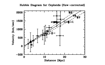
If the universe is expanding as depicted in Fig. 1.1, then galaxies should be moving away from each other. We should therefore see galaxies receding from us. Hubble (1929) first found that distant galaxies are in fact all apparently receding from us, i.e. redshifted. He also noticed the trend that the velocity increases with distance. This is exactly what we expect in an expanding universe, for the physical distance between two galaxies is $d=a x$ where $x$ is the comoving distance. ${ }^{1}$ In the absence of any comoving motion, $\dot{x} \equiv d x / d t=0$ (no peculiar velocity), the relative velocity $v$ is therefore equal to
$$
v=\frac{d}{d t}(a x)=\dot{a} x=H_{0} d \quad(v \ll c),
$$
where overdots indicate derivatives with respect to time $t$. Therefore, the apparent velocity should increase linearly with distance (at least at low redshift) with a slope given by $H_{0}$, the Hubble constant. Eq. (1.8) is known as the Hubble-Lemaitre law. The value of the constant is simply determined by measuring the slope of the line in the Hubble diagram shown in Fig. 1.5.

In the next chapter, we will generalize the distance-redshift relation to larger distances, where Eq. (1.8) breaks down. Instead of recession velocities, this more rigorous derivation will be based on the stretching of the wavelength of light encoded in Eq. (1.1). For now, let us just point out that the distance-redshift relation depends on the energy content of the universe. Data from a variety of sources point to a current best-fit scenario that is Euclidean and contains about $70 \%$ of the energy in the form of a cosmological constant, or some other form of dark energy. This now forms the concordance cosmology that will be our working model throughout.

宇宙学代考

物理代写|宇宙学代写cosmology代考|The concordance model of cosmology

爱因斯坦在上个世纪发现了广义相对论，这使我们在历史上第一次提出了一个令人信服的、可检验的宇宙理论。意识到宇宙正在膨胀并且曾经变得更热、更稠密，这让我们能够将古老的古老问题现代化，“我们为什么在这里？” “我们是怎么到这里的？” 现在更新的版本是“元素是如何形成的？”、“为什么宇宙如此光滑？”和“星系是如何在这个光滑的宇宙中形成的？” 值得注意的是，这些问题以及许多类似问题都有定量的答案，只有将我们的基础物理学知识与我们对早期宇宙条件的理解结合起来才能找到答案。更值得注意的是，这些答案可以通过天文观测来检验。在深入之前，
大爆炸范式的成功依赖于许多观测支柱：测量膨胀的哈勃图；与大爆炸核合成一致的轻元素丰度；宇宙微波背景中的温度和极化各向异性与理论非常吻合；和大尺度结构的多个探针也符合本章将要描述的一致性模型。然而，这种成功是有代价的：我们现在不得不引入超出粒子物理标准模型的几种成分（快速概览，见框 1.1）：

• 暗物质和暗能量，它们在宇宙生命的大部分时间里共同支配着宇宙的能量收支；
• 一种产生微小初始扰动的机制，形成结构，最流行的解释是暴胀。

物理代写|宇宙学代写cosmology代考|A nutshell history of the universe

我们有确凿的证据表明宇宙正在膨胀。这意味着在其历史早期，我们与遥远星系之间的距离比今天要小。通过引入比例因子可以方便地描述这种效果一个，其现值按惯例设置为 1。在更早的时候，一个比今天小。我们可以想象在空间中放置一个网格，如图 1.1 所示，它随着时间的推移均匀扩展。网格上的点，对应于静止的观察者，保持它们的坐标，所以两点之间的共同移动距离——它只是测量坐标之间的差异，可以通过计算网格单元来获得，如图 1.1 所示——保持不变。然而，物理距离与比例因子成正比，并且物理距离确实随着时间而变化。
一个直接相关的影响是，从远处物体发出的光的物理波长与比例因子成比例地拉伸，因此观察到的波长大于发出光的波长。将此拉伸因子定义为红移很方便和 :

1+和≡λ观测值 λ发射 =一个观测值 一个发射 =1一个发射 .
除了比例因子及其演化之外，光滑宇宙的特征还在于另一个参数，即它的几何形状。存在三种可能性：欧几里得宇宙、开放宇宙或封闭宇宙。这些不同的可能性最好通过考虑两个自由行进的粒子来理解，这两个粒子开始他们的旅程彼此平行移动。在欧几里得宇宙（通常也称为“平坦宇宙”）中，粒子的行为与欧几里得本人所期望的一样：只要它们自由行进，它们的轨迹就会保持平行。如果宇宙是封闭的，最初平行的粒子会逐渐收敛，就像在 2 球的情况下，所有恒经线在北极和南极相遇。封闭宇宙与球体表面的类比更深入：两者都是具有恒定正曲率的空间，前者在三个空间维度上，后者在两个空间维度上。最后，在一个开放的宇宙中，最初平行的路径会发散，就像两个大理石从马鞍上滚下来一样。

广义相对论将几何与能量联系起来。因此，宇宙中的总能量密度决定了几何形状：如果密度高于临界值，ρCr，我们很快就会看到大约是10−29 G C米−3，宇宙是封闭的；如果密度较低，则它是开放的。欧几里得宇宙是能量密度精确等于临界的宇宙。这似乎不太可能发生，但所有的观察都表明宇宙是欧几里得，误差范围内！稍后我们将看到通货膨胀为这一事实提供了一个自然的解释。

物理代写|宇宙学代写cosmology代考|The Hubble diagram

如果宇宙正在膨胀，如图 1.1 所示，那么星系应该彼此远离。因此，我们应该看到星系从我们身边退去。哈勃（1929）首先发现遥远的星系实际上都在明显地远离我们，即红移。他还注意到速度随距离增加的趋势。这正是我们在膨胀的宇宙中所期望的，因为两个星系之间的物理距离是d=一个X在哪里X是移动距离。1在没有任何同步运动的情况下，X˙≡dX/d吨=0（无特殊速度），相对速度在因此等于

在=dd吨(一个X)=一个˙X=H0d(在≪C),
其中过点表示关于时间的导数吨. 因此，视速度应随距离线性增加（至少在低红移处），其斜率由下式给出H0，哈勃常数。方程。(1.8) 被称为哈勃-勒梅特定律。通过测量图 1.5 所示的哈勃图中直线的斜率可以简单地确定常数的值。

在下一章中，我们将把距离-红移关系推广到更大的距离，其中方程式。(1.8) 崩溃。这种更严格的推导将基于方程式中编码的光波长的拉伸，而不是衰退速度。(1.1)。现在，让我们只指出距离-红移关系取决于宇宙的能量含量。来自各种来源的数据指向当前的最佳拟合方案，即欧几里得，包含约70%以宇宙常数或其他某种形式的暗能量形式的能量。这现在形成了和谐宇宙学，这将是我们自始至终的工作模型。

统计代写请认准statistics-lab™. statistics-lab™为您的留学生涯保驾护航。

金融工程代写

金融工程是使用数学技术来解决金融问题。金融工程使用计算机科学、统计学、经济学和应用数学领域的工具和知识来解决当前的金融问题，以及设计新的和创新的金融产品。

非参数统计代写

非参数统计指的是一种统计方法，其中不假设数据来自于由少数参数决定的规定模型；这种模型的例子包括正态分布模型和线性回归模型。

广义线性模型代考

广义线性模型（GLM）归属统计学领域，是一种应用灵活的线性回归模型。该模型允许因变量的偏差分布有除了正态分布之外的其它分布。

术语 广义线性模型（GLM）通常是指给定连续和/或分类预测因素的连续响应变量的常规线性回归模型。它包括多元线性回归，以及方差分析和方差分析（仅含固定效应）。

有限元方法代写

有限元方法（FEM）是一种流行的方法，用于数值解决工程和数学建模中出现的微分方程。典型的问题领域包括结构分析、传热、流体流动、质量运输和电磁势等传统领域。

有限元是一种通用的数值方法，用于解决两个或三个空间变量的偏微分方程（即一些边界值问题）。为了解决一个问题，有限元将一个大系统细分为更小、更简单的部分，称为有限元。这是通过在空间维度上的特定空间离散化来实现的，它是通过构建对象的网格来实现的：用于求解的数值域，它有有限数量的点。边界值问题的有限元方法表述最终导致一个代数方程组。该方法在域上对未知函数进行逼近。[1] 然后将模拟这些有限元的简单方程组合成一个更大的方程系统，以模拟整个问题。然后，有限元通过变化微积分使相关的误差函数最小化来逼近一个解决方案。

tatistics-lab作为专业的留学生服务机构，多年来已为美国、英国、加拿大、澳洲等留学热门地的学生提供专业的学术服务，包括但不限于Essay代写，Assignment代写，Dissertation代写，Report代写，小组作业代写，Proposal代写，Paper代写，Presentation代写，计算机作业代写，论文修改和润色，网课代做，exam代考等等。写作范围涵盖高中，本科，研究生等海外留学全阶段，辐射金融，经济学，会计学，审计学，管理学等全球99%专业科目。写作团队既有专业英语母语作者，也有海外名校硕博留学生，每位写作老师都拥有过硬的语言能力，专业的学科背景和学术写作经验。我们承诺100%原创，100%专业，100%准时，100%满意。

随机分析代写

随机微积分是数学的一个分支，对随机过程进行操作。它允许为随机过程的积分定义一个关于随机过程的一致的积分理论。这个领域是由日本数学家伊藤清在第二次世界大战期间创建并开始的。

时间序列分析代写

随机过程，是依赖于参数的一组随机变量的全体，参数通常是时间。 随机变量是随机现象的数量表现，其时间序列是一组按照时间发生先后顺序进行排列的数据点序列。通常一组时间序列的时间间隔为一恒定值（如1秒，5分钟，12小时，7天，1年），因此时间序列可以作为离散时间数据进行分析处理。研究时间序列数据的意义在于现实中，往往需要研究某个事物其随时间发展变化的规律。这就需要通过研究该事物过去发展的历史记录，以得到其自身发展的规律。

回归分析代写

多元回归分析渐进（Multiple Regression Analysis Asymptotics）属于计量经济学领域，主要是一种数学上的统计分析方法，可以分析复杂情况下各影响因素的数学关系，在自然科学、社会和经济学等多个领域内应用广泛。

MATLAB代写

MATLAB 是一种用于技术计算的高性能语言。它将计算、可视化和编程集成在一个易于使用的环境中，其中问题和解决方案以熟悉的数学符号表示。典型用途包括：数学和计算算法开发建模、仿真和原型制作数据分析、探索和可视化科学和工程图形应用程序开发，包括图形用户界面构建MATLAB 是一个交互式系统，其基本数据元素是一个不需要维度的数组。这使您可以解决许多技术计算问题，尤其是那些具有矩阵和向量公式的问题，而只需用 C 或 Fortran 等标量非交互式语言编写程序所需的时间的一小部分。MATLAB 名称代表矩阵实验室。MATLAB 最初的编写目的是提供对由 LINPACK 和 EISPACK 项目开发的矩阵软件的轻松访问，这两个项目共同代表了矩阵计算软件的最新技术。MATLAB 经过多年的发展，得到了许多用户的投入。在大学环境中，它是数学、工程和科学入门和高级课程的标准教学工具。在工业领域，MATLAB 是高效研究、开发和分析的首选工具。MATLAB 具有一系列称为工具箱的特定于应用程序的解决方案。对于大多数 MATLAB 用户来说非常重要，工具箱允许您学习和应用专业技术。工具箱是 MATLAB 函数（M 文件）的综合集合，可扩展 MATLAB 环境以解决特定类别的问题。可用工具箱的领域包括信号处理、控制系统、神经网络、模糊逻辑、小波、仿真等。

R语言代写	问卷设计与分析代写
PYTHON代写	回归分析与线性模型代写
MATLAB代写	方差分析与试验设计代写
STATA代写	机器学习/统计学习代写
SPSS代写	计量经济学代写
EVIEWS代写	时间序列分析代写
EXCEL代写	深度学习代写
SQL代写	各种数据建模与可视化代写

如果你也在 怎样代写宇宙学cosmology这个学科遇到相关的难题，请随时右上角联系我们的24/7代写客服。

宇宙学是天文学的一个分支，涉及宇宙的起源和演变，从大爆炸到今天，再到未来。宇宙学的定义是 “对整个宇宙的大尺度特性进行科学研究”。

statistics-lab™ 为您的留学生涯保驾护航 在代写宇宙学cosmology方面已经树立了自己的口碑, 保证靠谱, 高质且原创的统计Statistics代写服务。我们的专家在代写宇宙学cosmology代写方面经验极为丰富，各种代写宇宙学cosmology相关的作业也就用不着说。

我们提供的宇宙学cosmology及其相关学科的代写，服务范围广, 其中包括但不限于:

• Statistical Inference 统计推断
• Statistical Computing 统计计算
• Advanced Probability Theory 高等概率论
• Advanced Mathematical Statistics 高等数理统计学
• (Generalized) Linear Models 广义线性模型
• Statistical Machine Learning 统计机器学习
• Longitudinal Data Analysis 纵向数据分析
• Foundations of Data Science 数据科学基础

物理代写|宇宙学代写cosmology代考|Spherically symmetric gravitational fields

Spherical symmetry is a natural assumption in describing the simplest isolated bodies and island-like configurations. Spherically symmetric space-times are invariant under spatial rotations forming the isometry group G3.

In the general case, a spherically symmetric metric can be written in the form (see, e.g., [366])
$$
d s^{2}=\mathrm{e}^{2 \gamma} d t^{2}-\mathrm{e}^{2 \alpha} d u^{2}-\mathrm{e}^{2 \beta} d \Omega^{2}, \quad d \Omega^{2}=d \theta^{2}+\sin ^{2} \theta d \phi^{2},
$$
where $\alpha, \beta, \gamma$ are, in general, functions of the radial coordinate $u$ and the time coordinate $t$. We will also use the notation $r \equiv \mathrm{e}^{\beta}$; thus $r$ is the radius of a coordinate sphere $u=$ const, $t=$ const, and is also called the Schwarzschild radial coordinate, or the spherical radius, or, sometimes, the areal radius (since the area of such a coordinate sphere is equal to $4 \pi r^{2}$ ). In the expression (3.1), there is a freedom of choosing a reference frame (RF): different RFs correspond to spherically symmetric reference bodies with different radial velocity distributions with respect to each other.
The following two remarks are here in order.
First, let us note from the very beginning that in curved space the spherical radius $r$ has nothing to do with a distance to the center (as is the case in flat space), and in many spherically symmetric space-times there is no center at all.

Second, the “exponential” notations in (3.1) assume positive values of the corresponding metric coefficients. However, the quantities $g_{t t}$ and $g_{u u}$ can change their sign, and we will then accordingly change the notations.

物理代写|宇宙学代写cosmology代考|A regular center and asymptotic flatness

A center in a static, spherically symmetric space-time is, by definition, a point, line or surface in its spatial section where $r \equiv \mathrm{e}^{\beta}=0$,

that is, a place where coordinate spheres shrink to points. A center can be regular or singular; and regularity, as at any space-time point, is determined by finiteness of all $K_{i}$ in the expression (3.7). It is necessary to note that there can be no center at all in a spherically symmetric space-time; this happens if the quantity $r$ is nonzero in the whole space-time, or at least in its static region. We will encounter such behavior very soon, while discussing the properties of the Schwarzschild geometry.

With an arbitrary $u$ coordinate, the necessary and sufficient conditions for regularity of the metric at the center $(r=0)$ are obtained in the form
$$
\gamma=\gamma_{0}+O\left(r^{2}\right), \quad\left|\beta^{\prime}\right| \mathrm{e}^{-\alpha+\beta}=1+O\left(r^{2}\right)
$$
where $\gamma_{0}$ is a constant. The second condition is obtained from the finiteness requirement of the quantity $K_{4}$ in (3.7). Its meaning is that the circumference to radius ratio should take the correct value $(2 \pi)$ for small circles circumscribed around the center. This guarantees local flatness of space at the center and the existence of a tangent space. These are properties of any regular point – but for a center one has to introduce special regularity conditions because a center is a singular point of the class of spherical coordinate systems used.

物理代写|宇宙学代写cosmology代考|Solution of the Einstein equations

Let us find an important class of exact static, spherically symmetric solutions to the Einstein equations, characterizing the gravitational fields in vacuum or in the presence of an electromagnetic field (without charges) and a cosmological constant. This class contains the metrics that have the greatest number of astrophysical applications among all spherically symmetric metrics; it will also provide us with explicit examples in our future discussion of general properties of spherically symmetric space-times, including those with BHs.

It proves to be convenient to solve the problem in the curvature coordinates, in which two independent Einstein equations can be written in the form (3.5):
$$
\begin{aligned}
&G_{0}^{0}+\Lambda=\mathrm{e}^{-2 \alpha}\left(\frac{1}{r^{2}}-\frac{2 \alpha^{\prime}}{r}\right)-\frac{1}{r^{2}}+\Lambda=-\varkappa T_{0}^{0}, \
&G_{1}^{1}+\Lambda=\mathrm{e}^{-2 \alpha}\left(\frac{1}{r^{2}}+\frac{2 \gamma^{\prime}}{r}\right)-\frac{1}{r^{2}}+\Lambda=-\varkappa T_{1}^{1},
\end{aligned}
$$
where the prime denotes $d / d r$ while the SET in the present case corresponds to the electromagnetic field.
The Lagrangian and SET of the electromagnetic field are
$$
L_{\mathrm{e}-\mathrm{m}}=-\frac{1}{4} F_{\mu \nu} F^{\mu \nu}, \quad T_{\mu}^{\nu}=\frac{1}{4}\left[-4 F_{\mu \alpha} F^{\nu \alpha}+\delta_{\mu}^{\nu} F_{\alpha \beta} F^{\alpha \beta}\right] .
$$
The Maxwell equations $\nabla_{\alpha} F^{\alpha \beta}=0$ must now be written for the spherically symmetric case, so that among the components of $F_{\mu \nu}$ only the ones describing a radial electric field $\left(F_{01}=-F_{10}\right)$ and a radial magnetic field $\left(F_{23}=-F_{32}\right)$ can be nonzero. ${ }^{2}$ Let us restrict ourselves to an electric field. Then the only nontrivial Maxwell equation yields
$$
\left(\sqrt{-g} F^{01}\right)^{\prime}=0 \Rightarrow F^{01}=\frac{Q \mathrm{e}^{-\alpha-\gamma}}{\sqrt{4 \pi} r^{2}}, \quad F_{10}=\frac{Q \mathrm{e}^{\alpha+\gamma}}{\sqrt{4 \pi} r^{2}},
$$

宇宙学代考

物理代写|宇宙学代写cosmology代考|Spherically symmetric gravitational fields

球对称是描述最简单的孤立物体和岛状结构的自然假设。球对称时空在形成等距群 G3 的空间旋转下是不变的。

在一般情况下，球对称度量可以写成以下形式（参见，例如，[366]）

ds2=和2Cd吨2−和2一个d在2−和2bdΩ2,dΩ2=dθ2+罪2⁡θdφ2,
在哪里一个,b,C通常是径向坐标的函数在和时间坐标吨. 我们还将使用符号r≡和b; 因此r是坐标球的半径在=常量，吨=const，也称为 Schwarzschild 径向坐标，或球面半径，有时也称为面半径（因为这种坐标球面的面积等于4圆周率r2）。在表达式 (3.1) 中，存在选择参考系 (RF) 的自由度：不同的 RF 对应于具有不同径向速度分布的球对称参考体。
以下两点按顺序排列。
首先，让我们从一开始就注意到，在弯曲空间中，球面半径r与到中心的距离无关（就像在平坦空间中的情况），并且在许多球对称时空中根本没有中心。

其次，（3.1）中的“指数”符号假设相应度量系数的值为正。然而，数量G吨吨和G在在可以更改它们的符号，然后我们将相应地更改符号。

物理代写|宇宙学代写cosmology代考|A regular center and asymptotic flatness

根据定义，静态球对称时空中的中心是其空间截面中的点、线或面，其中r≡和b=0,

也就是坐标球收缩到点的地方。中心可以是规则的或单数的；和任何时空点一样，规律性是由所有的有限性决定的ķ一世在表达式 (3.7) 中。需要注意的是，在球对称的时空中根本不可能有中心；如果数量会发生这种情况r在整个时空中，或至少在其静态区域中是非零的。在讨论史瓦西几何的性质时，我们很快就会遇到这种行为。

以任意在坐标，中心度量正则的充要条件(r=0)以形式获得

C=C0+○(r2),|b′|和−一个+b=1+○(r2)
在哪里C0是一个常数。第二个条件是从数量的有限性要求中获得的ķ4在（3.7）中。它的意思是周长比应该取正确的值(2圆周率)对于围绕中心外接的小圆圈。这保证了中心空间的局部平坦度和切线空间的存在。这些是任何规则点的属性——但对于中心，必须引入特殊的规则条件，因为中心是所使用的球坐标系类的奇异点。

物理代写|宇宙学代写cosmology代考|Solution of the Einstein equations

让我们找到爱因斯坦方程的一类重要的精确静态球对称解，描述真空中或存在电磁场（不带电荷）和宇宙学常数时的引力场。此类包含所有球对称度量中天体物理学应用最多的度量；它还将在我们未来讨论球对称时空的一般性质时为我们提供明确的例子，包括那些具有 BH 的时空。

证明在曲率坐标中求解这个问题很方便，其中两个独立的爱因斯坦方程可以写成（3.5）形式：

G00+Λ=和−2一个(1r2−2一个′r)−1r2+Λ=−ε吨00, G11+Λ=和−2一个(1r2+2C′r)−1r2+Λ=−ε吨11,
其中素数表示d/dr而本例中的 SET 对应于电磁场。
电磁场的拉格朗日和 SET 是

大号和−米=−14FμνFμν,吨μν=14[−4Fμ一个Fν一个+dμνF一个bF一个b].
麦克斯韦方程∇一个F一个b=0现在必须写成球对称情况，所以在Fμν只有那些描述径向电场的(F01=−F10)和径向磁场(F23=−F32)可以是非零的。2让我们将自己限制在电场中。那么唯一的非平凡麦克斯韦方程产生

(−GF01)′=0⇒F01=问和−一个−C4圆周率r2,F10=问和一个+C4圆周率r2,

统计代写请认准statistics-lab™. statistics-lab™为您的留学生涯保驾护航。

金融工程代写

金融工程是使用数学技术来解决金融问题。金融工程使用计算机科学、统计学、经济学和应用数学领域的工具和知识来解决当前的金融问题，以及设计新的和创新的金融产品。

非参数统计代写

非参数统计指的是一种统计方法，其中不假设数据来自于由少数参数决定的规定模型；这种模型的例子包括正态分布模型和线性回归模型。

广义线性模型代考

广义线性模型（GLM）归属统计学领域，是一种应用灵活的线性回归模型。该模型允许因变量的偏差分布有除了正态分布之外的其它分布。

术语 广义线性模型（GLM）通常是指给定连续和/或分类预测因素的连续响应变量的常规线性回归模型。它包括多元线性回归，以及方差分析和方差分析（仅含固定效应）。

有限元方法代写

有限元方法（FEM）是一种流行的方法，用于数值解决工程和数学建模中出现的微分方程。典型的问题领域包括结构分析、传热、流体流动、质量运输和电磁势等传统领域。

有限元是一种通用的数值方法，用于解决两个或三个空间变量的偏微分方程（即一些边界值问题）。为了解决一个问题，有限元将一个大系统细分为更小、更简单的部分，称为有限元。这是通过在空间维度上的特定空间离散化来实现的，它是通过构建对象的网格来实现的：用于求解的数值域，它有有限数量的点。边界值问题的有限元方法表述最终导致一个代数方程组。该方法在域上对未知函数进行逼近。[1] 然后将模拟这些有限元的简单方程组合成一个更大的方程系统，以模拟整个问题。然后，有限元通过变化微积分使相关的误差函数最小化来逼近一个解决方案。

tatistics-lab作为专业的留学生服务机构，多年来已为美国、英国、加拿大、澳洲等留学热门地的学生提供专业的学术服务，包括但不限于Essay代写，Assignment代写，Dissertation代写，Report代写，小组作业代写，Proposal代写，Paper代写，Presentation代写，计算机作业代写，论文修改和润色，网课代做，exam代考等等。写作范围涵盖高中，本科，研究生等海外留学全阶段，辐射金融，经济学，会计学，审计学，管理学等全球99%专业科目。写作团队既有专业英语母语作者，也有海外名校硕博留学生，每位写作老师都拥有过硬的语言能力，专业的学科背景和学术写作经验。我们承诺100%原创，100%专业，100%准时，100%满意。

随机分析代写

随机微积分是数学的一个分支，对随机过程进行操作。它允许为随机过程的积分定义一个关于随机过程的一致的积分理论。这个领域是由日本数学家伊藤清在第二次世界大战期间创建并开始的。

时间序列分析代写

随机过程，是依赖于参数的一组随机变量的全体，参数通常是时间。 随机变量是随机现象的数量表现，其时间序列是一组按照时间发生先后顺序进行排列的数据点序列。通常一组时间序列的时间间隔为一恒定值（如1秒，5分钟，12小时，7天，1年），因此时间序列可以作为离散时间数据进行分析处理。研究时间序列数据的意义在于现实中，往往需要研究某个事物其随时间发展变化的规律。这就需要通过研究该事物过去发展的历史记录，以得到其自身发展的规律。

回归分析代写

多元回归分析渐进（Multiple Regression Analysis Asymptotics）属于计量经济学领域，主要是一种数学上的统计分析方法，可以分析复杂情况下各影响因素的数学关系，在自然科学、社会和经济学等多个领域内应用广泛。

MATLAB代写

MATLAB 是一种用于技术计算的高性能语言。它将计算、可视化和编程集成在一个易于使用的环境中，其中问题和解决方案以熟悉的数学符号表示。典型用途包括：数学和计算算法开发建模、仿真和原型制作数据分析、探索和可视化科学和工程图形应用程序开发，包括图形用户界面构建MATLAB 是一个交互式系统，其基本数据元素是一个不需要维度的数组。这使您可以解决许多技术计算问题，尤其是那些具有矩阵和向量公式的问题，而只需用 C 或 Fortran 等标量非交互式语言编写程序所需的时间的一小部分。MATLAB 名称代表矩阵实验室。MATLAB 最初的编写目的是提供对由 LINPACK 和 EISPACK 项目开发的矩阵软件的轻松访问，这两个项目共同代表了矩阵计算软件的最新技术。MATLAB 经过多年的发展，得到了许多用户的投入。在大学环境中，它是数学、工程和科学入门和高级课程的标准教学工具。在工业领域，MATLAB 是高效研究、开发和分析的首选工具。MATLAB 具有一系列称为工具箱的特定于应用程序的解决方案。对于大多数 MATLAB 用户来说非常重要，工具箱允许您学习和应用专业技术。工具箱是 MATLAB 函数（M 文件）的综合集合，可扩展 MATLAB 环境以解决特定类别的问题。可用工具箱的领域包括信号处理、控制系统、神经网络、模糊逻辑、小波、仿真等。

R语言代写	问卷设计与分析代写
PYTHON代写	回归分析与线性模型代写
MATLAB代写	方差分析与试验设计代写
STATA代写	机器学习/统计学习代写
SPSS代写	计量经济学代写
EVIEWS代写	时间序列分析代写
EXCEL代写	深度学习代写
SQL代写	各种数据建模与可视化代写

如果你也在 怎样代写宇宙学cosmology这个学科遇到相关的难题，请随时右上角联系我们的24/7代写客服。

宇宙学是天文学的一个分支，涉及宇宙的起源和演变，从大爆炸到今天，再到未来。宇宙学的定义是 “对整个宇宙的大尺度特性进行科学研究”。

statistics-lab™ 为您的留学生涯保驾护航 在代写宇宙学cosmology方面已经树立了自己的口碑, 保证靠谱, 高质且原创的统计Statistics代写服务。我们的专家在代写宇宙学cosmology代写方面经验极为丰富，各种代写宇宙学cosmology相关的作业也就用不着说。

我们提供的宇宙学cosmology及其相关学科的代写，服务范围广, 其中包括但不限于:

• Statistical Inference 统计推断
• Statistical Computing 统计计算
• Advanced Probability Theory 高等概率论
• Advanced Mathematical Statistics 高等数理统计学
• (Generalized) Linear Models 广义线性模型
• Statistical Machine Learning 统计机器学习
• Longitudinal Data Analysis 纵向数据分析
• Foundations of Data Science 数据科学基础

物理代写|宇宙学代写cosmology代考|Scalar fields

For a scalar field $\phi$ with arbitrary self-interaction, described by a potential $V(\phi)$, if it is minimally coupled to gravity, the Lagrangian in curved space is written in precisely the same way as in Minkowski space
$$
L_{s}=\frac{1}{2} g^{\mu \nu} \phi_{, \mu} \phi_{, \nu}-V(\phi),
$$
and its variation with respect to $\phi$ leads to an equation that generalizes the Klein-Gordon relativistic equation
$$
\square \phi+d V / d \phi=0,
$$
with the general-relativistic d’Alembert operator applied to a scalar
$$
\square=\nabla^{\alpha} \nabla_{\alpha}=\frac{1}{\sqrt{-g}} \partial_{\alpha}\left(\sqrt{-g} g^{\alpha \beta} \partial_{\beta}\right)
$$
(the same operator $\nabla^{\alpha} \nabla_{\alpha}$ applied to a vector or to a higher-rank tensor will have a more complicated expression due to more Christoffel symbols involved, see (2.34) and (2.37)).

The scalar field SET is obtained from the Lagrangian (2.72) by its variation according to (2.56):
$$
T_{\mu s}^{\nu}=\phi_{\mu} \phi^{\nu}-\delta_{\mu}^{\nu} L_{s} .
$$

More complex forms of scalar fields are also considered in the problems of gravitation and cosmology. For instance, the so-called $k$-essence with Lagrangians of the general form $L_{s}=L(\phi, X)$ (with $X=(\partial \phi)^{2}$ ) does not violate the minimal coupling principle.

Some of these Lagrangians as well as those with nonminimal coupling will be considered later.

物理代写|宇宙学代写cosmology代考|The electromagnetic field

The electromagnetic (massless vector) field is characterized by the vector potential $A_{\mu}$ and by the strength tensor, also called the Maxwell tensor
$$
F_{\mu \nu}=\partial_{\mu} A_{\nu}-\partial_{\nu} A_{\mu} .
$$
The electromagnetic field Lagrangian directly generalizes the corresponding flat-space expression. For a field with sources, the Lagrangian reads
$$
L_{\mathrm{e}-\mathrm{m}}=-\left(\frac{1}{4} F_{\mu \nu} F^{\mu \nu}-j^{\mu} A_{\mu}\right),
$$
where $j^{\mu}$ is the electric charge current density. Its variation with respect to $A_{\mu}$ gives a dynamic equation that corresponds to the second pair of Maxwell equations in usual electrodynamics,
$$
\nabla_{\nu} F^{\mu \nu} \equiv \frac{1}{\sqrt{-g}} \partial_{\nu}\left(\sqrt{-g} F^{\mu \nu}\right)=j^{\mu},
$$
and due to $(2.78)$, the electric charge conservation law automatically holds:
$$
\nabla_{\mu} j^{\mu} \equiv \frac{1}{\sqrt{-g}} \partial_{\mu}\left(\sqrt{-g} j^{\mu}\right)=0
$$
The first pair of Maxwell equations finds its analogue in the identity that follows from (2.76),
$$
\nabla_{\mu} F_{\nu \sigma}+\nabla_{\sigma} F_{\mu \nu}+\nabla_{\nu} F_{\sigma \mu}=0,
$$
or, equivalently,
$$
\nabla_{\mu}^{*} F^{\mu \nu}=0
$$

物理代写|宇宙学代写cosmology代考|Energy conditions

The energy conditions are certain invariant inequalities, mostly characterizing the known and conventional forms of matter, which are used in many studies and lead to many well-known results of outstanding significance, see, e.g., $[230,285,549]$. Let us enumerate and briefly discuss them.

Weak energy condition (WEC): Let $\xi^{\mu}$ be any timelike or null vector field $\left(\xi^{\mu} \xi_{\mu} \geq 0\right)$, and $T_{\mu \nu}$ the SET of matter or a particular kind of matter, then
$$
T_{\mu \nu} \xi^{\mu} \xi^{\nu} \geq 0 .
$$
If $\xi^{\mu}$ is timelike, we can choose the reference frame where this vector has the direction of 4 -velocity of matter, and then (2.84) reduces to $T_{0}^{0} \geq 0$, that is, the energy density of this kind of matter is nonnegative.

If $\xi^{\mu}$ is null, then the inequality (2.84) has its own separate name.
Null energy condition (NEC): It is the inequality whose violation is a necessary condition at wormhole throats in GR and other “exotic” objects and phantom dark energy in cosmology. If $T_{\mu \nu}$ is the SET of an anisotropic fluid $(2.68)$ in its comoving frame, then (2.84) takes the form
$$
\rho+p_{i} \geq 0, \quad i=1,2,3
$$
Example: The cosmological constant $\Lambda>0$, if treated as a kind of matter, satisfies the WEC, but respects the NEC only marginally since for it $\rho=\Lambda$ and $p=-\Lambda$.

宇宙学代考

物理代写|宇宙学代写cosmology代考|Scalar fields

对于标量场φ具有任意自交互作用，由势能描述在(φ)，如果它与重力最小耦合，则弯曲空间中的拉格朗日函数的写法与 Minkowski 空间中的写法完全相同

大号s=12Gμνφ,μφ,ν−在(φ),
及其变化相对于φ导致一个方程推广了克莱因-戈登相对论方程

φ+d在/dφ=0,
将广义相对论 d’Alembert 算子应用于标量

=∇一个∇一个=1−G∂一个(−GG一个b∂b)
（同一个运算符∇一个∇一个由于涉及更多 Christoffel 符号，应用于向量或更高阶张量将具有更复杂的表达式，请参见 (2.34) 和 (2.37))。

标量场 SET 是从拉格朗日算子 (2.72) 通过其根据 (2.56) 的变化获得的：

吨μsν=φμφν−dμν大号s.

在引力和宇宙学问题中也考虑了更复杂形式的标量场。例如，所谓的ķ- 具有一般形式的拉格朗日量的本质大号s=大号(φ,X)（和X=(∂φ)2) 不违反最小耦合原则。

稍后将考虑其中一些拉格朗日算子以及具有非最小耦合的拉格朗日算子。

物理代写|宇宙学代写cosmology代考|The electromagnetic field

电磁（无质量矢量）场的特征在于矢量势一个μ并由强度张量，也称为麦克斯韦张量

Fμν=∂μ一个ν−∂ν一个μ.
电磁场拉格朗日直接推广了相应的平面空间表达式。对于有源的字段，拉格朗日函数读取

大号和−米=−(14FμνFμν−jμ一个μ),
在哪里jμ是电荷电流密度。它的变化相对于一个μ给出对应于通常电动力学中的第二对麦克斯韦方程组的动力学方程，

∇νFμν≡1−G∂ν(−GFμν)=jμ,
并且由于(2.78)，电荷守恒定律自动成立：

∇μjμ≡1−G∂μ(−Gjμ)=0
第一对麦克斯韦方程组在 (2.76) 的恒等式中找到它的类似物，

∇μFνσ+∇σFμν+∇νFσμ=0,
或者，等效地，

∇μ∗Fμν=0

物理代写|宇宙学代写cosmology代考|Energy conditions

能量条件是某些不变的不等式，主要表征已知和常规形式的物质，它们被用于许多研究并导致许多具有突出意义的众所周知的结果，例如，[230,285,549]. 让我们列举并简要讨论它们。

弱能条件（WEC）：让Xμ是任何类时或空向量场(XμXμ≥0)， 和吨μν物质的集合或特定种类的物质，那么

吨μνXμXν≥0.
如果Xμ是时间似的，我们可以选择这个向量的方向是物质速度为 4 的参考系，然后 (2.84) 简化为吨00≥0，即这种物质的能量密度是非负的。

如果Xμ为空，则不等式 (2.84) 有自己的独立名称。
零能量条件（NEC）：它是不等式，它的违反是 GR 和其他“奇异”物体的虫洞喉部和宇宙学中的幻影暗能量的必要条件。如果吨μν是各向异性流体的 SET(2.68)那么 (2.84) 在它的同动框架中的形式为

ρ+p一世≥0,一世=1,2,3
例子：宇宙常数Λ>0，如果被视为一种事物，则满足 WEC，但仅略微尊重 NEC，因为它ρ=Λ和p=−Λ.

统计代写请认准statistics-lab™. statistics-lab™为您的留学生涯保驾护航。

金融工程代写

金融工程是使用数学技术来解决金融问题。金融工程使用计算机科学、统计学、经济学和应用数学领域的工具和知识来解决当前的金融问题，以及设计新的和创新的金融产品。

非参数统计代写

非参数统计指的是一种统计方法，其中不假设数据来自于由少数参数决定的规定模型；这种模型的例子包括正态分布模型和线性回归模型。

广义线性模型代考

广义线性模型（GLM）归属统计学领域，是一种应用灵活的线性回归模型。该模型允许因变量的偏差分布有除了正态分布之外的其它分布。

术语 广义线性模型（GLM）通常是指给定连续和/或分类预测因素的连续响应变量的常规线性回归模型。它包括多元线性回归，以及方差分析和方差分析（仅含固定效应）。

有限元方法代写

有限元方法（FEM）是一种流行的方法，用于数值解决工程和数学建模中出现的微分方程。典型的问题领域包括结构分析、传热、流体流动、质量运输和电磁势等传统领域。

有限元是一种通用的数值方法，用于解决两个或三个空间变量的偏微分方程（即一些边界值问题）。为了解决一个问题，有限元将一个大系统细分为更小、更简单的部分，称为有限元。这是通过在空间维度上的特定空间离散化来实现的，它是通过构建对象的网格来实现的：用于求解的数值域，它有有限数量的点。边界值问题的有限元方法表述最终导致一个代数方程组。该方法在域上对未知函数进行逼近。[1] 然后将模拟这些有限元的简单方程组合成一个更大的方程系统，以模拟整个问题。然后，有限元通过变化微积分使相关的误差函数最小化来逼近一个解决方案。

tatistics-lab作为专业的留学生服务机构，多年来已为美国、英国、加拿大、澳洲等留学热门地的学生提供专业的学术服务，包括但不限于Essay代写，Assignment代写，Dissertation代写，Report代写，小组作业代写，Proposal代写，Paper代写，Presentation代写，计算机作业代写，论文修改和润色，网课代做，exam代考等等。写作范围涵盖高中，本科，研究生等海外留学全阶段，辐射金融，经济学，会计学，审计学，管理学等全球99%专业科目。写作团队既有专业英语母语作者，也有海外名校硕博留学生，每位写作老师都拥有过硬的语言能力，专业的学科背景和学术写作经验。我们承诺100%原创，100%专业，100%准时，100%满意。

随机分析代写

随机微积分是数学的一个分支，对随机过程进行操作。它允许为随机过程的积分定义一个关于随机过程的一致的积分理论。这个领域是由日本数学家伊藤清在第二次世界大战期间创建并开始的。

时间序列分析代写

随机过程，是依赖于参数的一组随机变量的全体，参数通常是时间。 随机变量是随机现象的数量表现，其时间序列是一组按照时间发生先后顺序进行排列的数据点序列。通常一组时间序列的时间间隔为一恒定值（如1秒，5分钟，12小时，7天，1年），因此时间序列可以作为离散时间数据进行分析处理。研究时间序列数据的意义在于现实中，往往需要研究某个事物其随时间发展变化的规律。这就需要通过研究该事物过去发展的历史记录，以得到其自身发展的规律。

回归分析代写

多元回归分析渐进（Multiple Regression Analysis Asymptotics）属于计量经济学领域，主要是一种数学上的统计分析方法，可以分析复杂情况下各影响因素的数学关系，在自然科学、社会和经济学等多个领域内应用广泛。

MATLAB代写

MATLAB 是一种用于技术计算的高性能语言。它将计算、可视化和编程集成在一个易于使用的环境中，其中问题和解决方案以熟悉的数学符号表示。典型用途包括：数学和计算算法开发建模、仿真和原型制作数据分析、探索和可视化科学和工程图形应用程序开发，包括图形用户界面构建MATLAB 是一个交互式系统，其基本数据元素是一个不需要维度的数组。这使您可以解决许多技术计算问题，尤其是那些具有矩阵和向量公式的问题，而只需用 C 或 Fortran 等标量非交互式语言编写程序所需的时间的一小部分。MATLAB 名称代表矩阵实验室。MATLAB 最初的编写目的是提供对由 LINPACK 和 EISPACK 项目开发的矩阵软件的轻松访问，这两个项目共同代表了矩阵计算软件的最新技术。MATLAB 经过多年的发展，得到了许多用户的投入。在大学环境中，它是数学、工程和科学入门和高级课程的标准教学工具。在工业领域，MATLAB 是高效研究、开发和分析的首选工具。MATLAB 具有一系列称为工具箱的特定于应用程序的解决方案。对于大多数 MATLAB 用户来说非常重要，工具箱允许您学习和应用专业技术。工具箱是 MATLAB 函数（M 文件）的综合集合，可扩展 MATLAB 环境以解决特定类别的问题。可用工具箱的领域包括信号处理、控制系统、神经网络、模糊逻辑、小波、仿真等。

R语言代写	问卷设计与分析代写
PYTHON代写	回归分析与线性模型代写
MATLAB代写	方差分析与试验设计代写
STATA代写	机器学习/统计学习代写
SPSS代写	计量经济学代写
EVIEWS代写	时间序列分析代写
EXCEL代写	深度学习代写
SQL代写	各种数据建模与可视化代写

如果你也在 怎样代写宇宙学cosmology这个学科遇到相关的难题，请随时右上角联系我们的24/7代写客服。

宇宙学是天文学的一个分支，涉及宇宙的起源和演变，从大爆炸到今天，再到未来。宇宙学的定义是 “对整个宇宙的大尺度特性进行科学研究”。

statistics-lab™ 为您的留学生涯保驾护航 在代写宇宙学cosmology方面已经树立了自己的口碑, 保证靠谱, 高质且原创的统计Statistics代写服务。我们的专家在代写宇宙学cosmology代写方面经验极为丰富，各种代写宇宙学cosmology相关的作业也就用不着说。

我们提供的宇宙学cosmology及其相关学科的代写，服务范围广, 其中包括但不限于:

• Statistical Inference 统计推断
• Statistical Computing 统计计算
• Advanced Probability Theory 高等概率论
• Advanced Mathematical Statistics 高等数理统计学
• (Generalized) Linear Models 广义线性模型
• Statistical Machine Learning 统计机器学习
• Longitudinal Data Analysis 纵向数据分析
• Foundations of Data Science 数据科学基础

物理代写|宇宙学代写cosmology代考|The correspondence principle

Since a Riemannian space-time coincides with Minkowski space (its tangent space) in a small vicinity of each world point, the laws of SR are approximately valid at any point. It is possible to pass on to SR in the whole space in the limit of weak gravity; the weak gravity condition is formulated as the condition that the metric is only weakly deflecting from the flat metric (in any coordinates), or that the Riemann tensor is small in terms of a certain length scale.

It should be noted, however, that the formal transition $x \rightarrow 0$ in a solution to the Einstein equations does not generally lead to a flat metric: instead, it leads to a certain nonflat vacuum solution of the Einstein equations, that is, a solution with $T_{\mu \nu} \equiv 0$.

Newton’s law of gravity follows from GR under the conditions of small velocities $(v \ll c$ ) and weak gravity (that is, the Newtonian gravitational potential, introduced in a proper way, should be small, $V \ll c^{2}$ ). In what follows, we shall verify the existence of such a transition using as an example the Schwarzschild metric, and also the validity of the relation $x=8 \pi G / c^{4}$.

A transition to Newtonian gravity can also be carried out under some additional conditions by the formal transition $c \rightarrow \infty$, and an expansion of the metric in powers of $c^{-1}$ (more precisely, in powers of $v / c$ and $V / c^{2}$ ). Such an expansion of the metric tensor is convenient for describing the observable effects of relativistic gravity in weak gravitational fields (for example, in the Solar system) by using a few first terms. This tool is applicable both in GR (the postNewtonian approximation) and in other metric theories of gravity (the parametrized post-Newtonian (PPN) approximation) [563]. For example, in the first PPN approximation the component $g_{00}$ should be calculated up to $c^{-4}$ (since it is multiplied by $c^{2} d t^{2}$ ), the components $g_{0 i}$ up to $c^{-3}$, and the components $g_{i j}$ up to $c^{-2}$. Higher-order PPN coefficients are also in demand owing to the increasing accuracy of measurements [565].

物理代写|宇宙学代写cosmology代考|Macroscopic matter and nongravitational

All kinds of matter other than the gravitational field admit a description in the framework of SR. For their description in GR (and, in general, in any theory formulated in a Riemannian space), most frequently (but not always), the so-called minimal coupling principle is used, according to which all equations known in SR are extended to curved space time by replacing all partial derivatives with covariant derivatives. We note that this trick can even increase the freedom of calculations in the framework of SR without restriction to Minkowski

coordinates, introducing curvilinear coordinates and invoking any accelerations, both translational and rotational ones.

We will present some relations valid for nongravitational matter in curved space-time according to the minimal coupling principle.

物理代写|宇宙学代写cosmology代考|Perfect fluids

We have previously presented the expression (2.59) for the SET of a perfect fluid in Riemannian space-time in a derivation of the geodesic equations. Let us now consider a more general conservation law for a perfect fluid and derive the corresponding equations of motion, the general-relativistic analogues of the continuity equation and the Euler equation.
Rewrite the tensor (2.59) in mixed components,
$$
T_{\mu}^{\nu}=(\varepsilon+p) u_{\mu} u^{\nu}-p \delta_{\mu}^{\nu},
$$
apply to it the operator $\nabla_{\nu}$ and equate the result to zero
$$
\nabla_{\nu} T_{\mu}^{\nu}=\left(\partial_{\nu} w\right) u_{\mu} u^{\nu}+w \nabla_{\nu}\left(u_{\mu} u^{\nu}\right)-\partial_{\mu} p=0
$$
where $w:=\varepsilon+p$ is the thermal function of the fluid. Contracting (2.64) with $u^{\mu}$ (i.e., finding its projection to the direction of $u^{\mu}$ ) and recalling that $\partial_{\mu}\left(u_{\nu} u^{\nu}\right)=0$, we obtain
$$
\nabla_{\nu}\left(w u^{\nu}\right)-u^{\mu} \partial_{\mu} p=0
$$
Let us now make a projection of (2.64) onto a direction perpendicular to $u^{\mu}$. Such a projection has the form $\nabla_{\nu} T_{\mu}^{\nu}-u^{\nu} u_{\mu} \nabla_{\lambda} T_{\nu}^{\lambda}=0$. As a result, we arrive at the perfect fluid equation of motion, the generalrelativistic analogue of the Euler equation
$$
w u^{\nu} \nabla_{\nu} u_{\mu}=\partial_{\mu} p-u_{\mu} u^{\nu} \partial_{\nu} p
$$
In nonrelativistic hydrodynamics, the continuity equation is known to represent the mass conservation law. In SR and, even more in GR, the mass is not conserved, and analogues of the continuity equation are only obtained for conserved quantities such as the number of particles if one can neglect their possible production and absorption. Then one can introduce the particle number current $n^{\mu}=n u^{\mu}$, where $n$ is the particle number density in the RF where the fluid formed by these particles is at rest, and $u^{\mu}$ is the 4-velocity of this fluid. The particle number conservation law (valid in the absence of their creation, annihilation and conversion) is expressed in the equality
$$
\nabla_{\mu}\left(n u^{\mu}\right)=0,
$$
quite similar to the electric charge conservation law (2.79) (see below).

宇宙学代考

物理代写|宇宙学代写cosmology代考|The correspondence principle

由于黎曼时空与闵可夫斯基空间（其切线空间）在每个世界点附近的一小部分重合，因此 SR 定律在任何点都近似有效。在弱重力的限制下，可以全空间传递给SR；弱重力条件被表述为度量仅从平面度量（在任何坐标中）弱偏转的条件，或者黎曼张量在一定长度尺度方面很小。

但需要注意的是，正式的过渡X→0爱因斯坦方程的解通常不会导致平坦度量：相反，它会导致爱因斯坦方程的某个非平坦真空解，即吨μν≡0.

牛顿万有引力定律在小速度条件下由 GR 得出(在≪C）和弱引力（即牛顿引力势，以适当的方式引入，应该很小，在≪C2）。在下文中，我们将使用 Schwarzschild 度量作为示例来验证这种转换的存在，以及关系的有效性X=8圆周率G/C4.

在一些额外的条件下，也可以通过正式的转变来实现向牛顿引力的转变C→∞，以及度量的扩展C−1（更准确地说，在权力在/C和在/C2）。度量张量的这种扩展通过使用一些第一项，便于描述相对论引力在弱引力场（例如，在太阳系中）中的可观测效应。该工具适用于 GR（后牛顿近似）和其他度量引力理论（参数化后牛顿 (PPN) 近似）[563]。例如，在第一个 PPN 近似中，分量G00应该计算到C−4（因为它乘以C2d吨2), 组件G0一世取决于C−3, 和组件G一世j取决于C−2. 由于测量精度的提高，也需要高阶 PPN 系数 [565]。

物理代写|宇宙学代写cosmology代考|Macroscopic matter and nongravitational

引力场以外的所有物质都可以在 SR 的框架内进行描述。对于它们在 GR 中的描述（以及通常在黎曼空间中表述的任何理论），最常见（但不总是）使用所谓的最小耦合原理，根据该原理，SR 中已知的所有方程都可以扩展到通过用协变导数替换所有偏导数来弯曲时空。我们注意到，这个技巧甚至可以增加 SR 框架中的计算自由度，而不受 Minkowski 的限制

坐标，引入曲线坐标并调用任何加速度，包括平移和旋转加速度。

我们将根据最小耦合原理提出一些适用于弯曲时空中的非引力物质的关系。

物理代写|宇宙学代写cosmology代考|Perfect fluids

我们之前在测地线方程的推导中提出了黎曼时空中完美流体的 SET 的表达式 (2.59)。现在让我们考虑一个更一般的完美流体守恒定律，并推导出相应的运动方程、连续性方程和欧拉方程的广义相对论类似物。
用混合分量重写张量（2.59），

吨μν=(e+p)在μ在ν−pdμν,
适用于它的运营商∇ν并将结果等同于零

∇ν吨μν=(∂ν在)在μ在ν+在∇ν(在μ在ν)−∂μp=0
在哪里在:=e+p是流体的热函数。与 (2.64) 签约在μ（即，找到它的投影方向在μ) 并回忆起∂μ(在ν在ν)=0， 我们获得

∇ν(在在ν)−在μ∂μp=0
现在让我们将 (2.64) 投影到垂直于在μ. 这样的投影具有以下形式∇ν吨μν−在ν在μ∇λ吨νλ=0. 结果，我们得到了完美的流体运动方程，即欧拉方程的广义相对论模拟

在在ν∇ν在μ=∂μp−在μ在ν∂νp
在非相对论流体动力学中，已知连续性方程代表质量守恒定律。在 SR 中，甚至在 GR 中，质量不是守恒的，如果可以忽略粒子可能的产生和吸收，则只能针对诸如粒子数之类的守恒量获得连续性方程的类似物。那么可以引入粒子数电流nμ=n在μ， 在哪里n是由这些粒子形成的流体处于静止状态的 RF 中的粒子数密度，并且在μ是这种流体的 4 速度。粒子数守恒定律（在没有它们的创造、湮灭和转换的情况下有效）表示为等式

∇μ(n在μ)=0,
非常类似于电荷守恒定律（2.79）（见下文）。

统计代写请认准statistics-lab™. statistics-lab™为您的留学生涯保驾护航。

金融工程代写

金融工程是使用数学技术来解决金融问题。金融工程使用计算机科学、统计学、经济学和应用数学领域的工具和知识来解决当前的金融问题，以及设计新的和创新的金融产品。

非参数统计代写

非参数统计指的是一种统计方法，其中不假设数据来自于由少数参数决定的规定模型；这种模型的例子包括正态分布模型和线性回归模型。

广义线性模型代考

广义线性模型（GLM）归属统计学领域，是一种应用灵活的线性回归模型。该模型允许因变量的偏差分布有除了正态分布之外的其它分布。

术语 广义线性模型（GLM）通常是指给定连续和/或分类预测因素的连续响应变量的常规线性回归模型。它包括多元线性回归，以及方差分析和方差分析（仅含固定效应）。

有限元方法代写

有限元方法（FEM）是一种流行的方法，用于数值解决工程和数学建模中出现的微分方程。典型的问题领域包括结构分析、传热、流体流动、质量运输和电磁势等传统领域。

有限元是一种通用的数值方法，用于解决两个或三个空间变量的偏微分方程（即一些边界值问题）。为了解决一个问题，有限元将一个大系统细分为更小、更简单的部分，称为有限元。这是通过在空间维度上的特定空间离散化来实现的，它是通过构建对象的网格来实现的：用于求解的数值域，它有有限数量的点。边界值问题的有限元方法表述最终导致一个代数方程组。该方法在域上对未知函数进行逼近。[1] 然后将模拟这些有限元的简单方程组合成一个更大的方程系统，以模拟整个问题。然后，有限元通过变化微积分使相关的误差函数最小化来逼近一个解决方案。

tatistics-lab作为专业的留学生服务机构，多年来已为美国、英国、加拿大、澳洲等留学热门地的学生提供专业的学术服务，包括但不限于Essay代写，Assignment代写，Dissertation代写，Report代写，小组作业代写，Proposal代写，Paper代写，Presentation代写，计算机作业代写，论文修改和润色，网课代做，exam代考等等。写作范围涵盖高中，本科，研究生等海外留学全阶段，辐射金融，经济学，会计学，审计学，管理学等全球99%专业科目。写作团队既有专业英语母语作者，也有海外名校硕博留学生，每位写作老师都拥有过硬的语言能力，专业的学科背景和学术写作经验。我们承诺100%原创，100%专业，100%准时，100%满意。

随机分析代写

随机微积分是数学的一个分支，对随机过程进行操作。它允许为随机过程的积分定义一个关于随机过程的一致的积分理论。这个领域是由日本数学家伊藤清在第二次世界大战期间创建并开始的。

时间序列分析代写

随机过程，是依赖于参数的一组随机变量的全体，参数通常是时间。 随机变量是随机现象的数量表现，其时间序列是一组按照时间发生先后顺序进行排列的数据点序列。通常一组时间序列的时间间隔为一恒定值（如1秒，5分钟，12小时，7天，1年），因此时间序列可以作为离散时间数据进行分析处理。研究时间序列数据的意义在于现实中，往往需要研究某个事物其随时间发展变化的规律。这就需要通过研究该事物过去发展的历史记录，以得到其自身发展的规律。

回归分析代写

多元回归分析渐进（Multiple Regression Analysis Asymptotics）属于计量经济学领域，主要是一种数学上的统计分析方法，可以分析复杂情况下各影响因素的数学关系，在自然科学、社会和经济学等多个领域内应用广泛。

MATLAB代写

MATLAB 是一种用于技术计算的高性能语言。它将计算、可视化和编程集成在一个易于使用的环境中，其中问题和解决方案以熟悉的数学符号表示。典型用途包括：数学和计算算法开发建模、仿真和原型制作数据分析、探索和可视化科学和工程图形应用程序开发，包括图形用户界面构建MATLAB 是一个交互式系统，其基本数据元素是一个不需要维度的数组。这使您可以解决许多技术计算问题，尤其是那些具有矩阵和向量公式的问题，而只需用 C 或 Fortran 等标量非交互式语言编写程序所需的时间的一小部分。MATLAB 名称代表矩阵实验室。MATLAB 最初的编写目的是提供对由 LINPACK 和 EISPACK 项目开发的矩阵软件的轻松访问，这两个项目共同代表了矩阵计算软件的最新技术。MATLAB 经过多年的发展，得到了许多用户的投入。在大学环境中，它是数学、工程和科学入门和高级课程的标准教学工具。在工业领域，MATLAB 是高效研究、开发和分析的首选工具。MATLAB 具有一系列称为工具箱的特定于应用程序的解决方案。对于大多数 MATLAB 用户来说非常重要，工具箱允许您学习和应用专业技术。工具箱是 MATLAB 函数（M 文件）的综合集合，可扩展 MATLAB 环境以解决特定类别的问题。可用工具箱的领域包括信号处理、控制系统、神经网络、模糊逻辑、小波、仿真等。

R语言代写	问卷设计与分析代写
PYTHON代写	回归分析与线性模型代写
MATLAB代写	方差分析与试验设计代写
STATA代写	机器学习/统计学习代写
SPSS代写	计量经济学代写
EVIEWS代写	时间序列分析代写
EXCEL代写	深度学习代写
SQL代写	各种数据建模与可视化代写

如果你也在 怎样代写宇宙学cosmology这个学科遇到相关的难题，请随时右上角联系我们的24/7代写客服。

宇宙学是天文学的一个分支，涉及宇宙的起源和演变，从大爆炸到今天，再到未来。宇宙学的定义是 “对整个宇宙的大尺度特性进行科学研究”。

statistics-lab™ 为您的留学生涯保驾护航 在代写宇宙学cosmology方面已经树立了自己的口碑, 保证靠谱, 高质且原创的统计Statistics代写服务。我们的专家在代写宇宙学cosmology代写方面经验极为丰富，各种代写宇宙学cosmology相关的作业也就用不着说。

我们提供的宇宙学cosmology及其相关学科的代写，服务范围广, 其中包括但不限于:

• Statistical Inference 统计推断
• Statistical Computing 统计计算
• Advanced Probability Theory 高等概率论
• Advanced Mathematical Statistics 高等数理统计学
• (Generalized) Linear Models 广义线性模型
• Statistical Machine Learning 统计机器学习
• Longitudinal Data Analysis 纵向数据分析
• Foundations of Data Science 数据科学基础

物理代写|宇宙学代写cosmology代考|Riemannian space–time — curvature

Let us present some definitions and relations, important for the further content of the book.

To begin with, the contravariant components of the metric $g^{\mu \nu}$ form a matrix reciprocal to the matrix $g_{\mu \nu}$ :
$$
g_{\mu \alpha} g^{\alpha \nu}=\delta_{\mu}^{\nu},
$$

where $\delta_{\mu}^{\nu}$ is the Kronecker symbol, a tensor whose components form the unity matrix: they are equal to unity for coinciding values of the indices and to zero for noncoinciding ones. The tensors $g_{\mu \nu}$ and $g^{\mu \nu}$ are used for raising and lowering arbitrary tensor indices.

Partial derivatives of any scalar function (that is, a function whose values are the same in all coordinate systems) $f\left(x^{\mu}\right)$ with respect to the coordinates, $\partial_{\mu} f$, form a covariant vector called the gradient of $f$. Partial derivatives of the components of a vector $A_{\mu}$ or $A^{\mu}$, in general, do not form a tensor because coordinate transformations are, in general, nonlinear. To obtain a covariant form of physical equations and for many other purposes it is thus necessary to generalize the notion of a derivative, to make it a tensor. This goal is achieved by introducing the covariant derivatives
$$
\begin{aligned}
&\nabla_{\mu} A_{\nu}=\partial_{\mu} A_{\nu}-\Gamma_{\mu \nu}^{\alpha} A_{\alpha} \
&\nabla_{\mu} A^{\nu}=\partial_{\mu} A^{\nu}+\Gamma_{\mu \alpha}^{\nu} A^{\alpha}
\end{aligned}
$$
where the quantities $\Gamma_{\mu \nu}^{\alpha}$ (they do not form a tensor!) are called the Christoffel symbols, or affine connection coefficients agreeing with the metric (the metric connection, or the metric affinity). They are expressed in terms of the metric tensor and its first-order partial derivatives:
$$
\Gamma_{\mu \nu}^{\sigma}=\frac{1}{2} g^{\sigma \alpha}\left(\partial_{\nu} g_{\alpha \mu}+\partial_{\mu} g_{\alpha \nu}-\partial_{\alpha} g_{\mu \nu}\right)
$$

物理代写|宇宙学代写cosmology代考|The Einstein equations

In GR, the dynamic variables characterizing the gravitational field are the metric tensor components $g_{\mu \nu}$. The dynamic equations of GR are derived from Hilbert’s variation principle
$$
\delta S=0, \quad S=\int \frac{R-2 \Lambda}{2 x} \sqrt{-g} d^{4} x+S_{m},
$$
where $S_{m}=\int L_{m} \sqrt{-g} d^{4} x$ is the action of matter, i.e., substance and all fields except the gravitational field, and $\Lambda$ is the cosmological constant, which is usually negligible when considering “local” configurations (up to the scale of a cluster of galaxies) but is manifestly important on the cosmological scale. The condition $\delta S=0$ leads to the Hilbert-Einstein equations (more frequently they are simply called the Einstein equations)
$$
R_{\mu \nu}-\frac{1}{2} g_{\mu \nu} R+g_{\mu \nu} \Lambda=-\varkappa T_{\mu \nu} .
$$
Here, $\varkappa=8 \pi G / c^{4}$ is the Einstein gravitational constant ( $G$ is the Newtonian gravitational constant), and $T_{\mu \nu}$ is the (metric) stressenergy tensor (SET) of matter:
$$
T_{\mu \nu}=\frac{2}{\sqrt{-g}} \frac{\delta S_{m}}{\delta g^{\mu \nu}} .
$$
In (2.55), there are in general ten nonlinear partial differential equations. However, first, the freedom of choosing a coordinate system makes it possible to impose four arbitrary coordinate conditions which can be formulated as equalities involving the coefficients $g_{\mu \nu}$, and therefore remain only six independent equations. Second, among the remaining equations there are four differential dependences related to the identities (2.46), which results in only two real dynamic equations. The other four are constraint equations which do not contain second-order time derivatives. These circumstances are of importance for all dynamic processes in GR, and above all for gravitational waves, which can have only two independent polarizations.

物理代写|宇宙学代写cosmology代考|Geodesic equations

The equations of motion for free particles in Riemannian space-times can be obtained by varying the action (2.21) (now written for a Riemannian linear element). The variation equation, as in Minkowski space, has the meaning of a trajectory (geodesic) equation, describing the extremum of the world line length between two given points. It can be written as
$$
\frac{d u^{\alpha}}{d s}+\Gamma_{\mu \nu}^{\alpha} u^{\mu} u^{\nu}=0 .
$$
Here, $s$ is the interval which coincides with the proper time of an observer moving along the geodesic if it is timelike and the proper length along the geodesic if it is spacelike. In all cases $s$ is a canonical parameter. ${ }^{5}$

Let us derive Eq. (2.58) from the conservation law (2.57). It will be a good illustration of the possibility to derive the equations of motion for matter from the Einstein equations.

Let us begin with the expression for the SET of a perfect fluid, which can be obtained as a natural extension of the corresponding expression from SR [366] to Riemannian spaces:
$$
T_{\mu \nu}=(\varepsilon+p) u_{\mu} u_{\nu}-p g_{\mu \nu},
$$

where $u_{\mu}$ is the 4 -velocity of particles of the fluid, $\varepsilon=\rho c^{2}$ is its energy density, and $p$ its pressure. In particular, for dustlike matter, consisting of noninteracting particles,
$$
p=0, \quad T_{\mu \nu}=\varepsilon u_{\mu} u_{\nu}
$$

宇宙学代考

物理代写|宇宙学代写cosmology代考|Riemannian space–time — curvature

让我们提出一些定义和关系，这对本书的进一步内容很重要。

首先，度量的逆变分量gμν形成矩阵的倒数矩阵gμν :

gμαgαν=δμν,

在哪里δμν是克罗内克符号，一个张量，其分量构成单位矩阵：对于一致的索引值，它们等于单位，对于不重合的值，它们等于零。张量gμν和gμν用于提高和降低任意张量指数。

任何标量函数的偏导数（即在所有坐标系中值都相同的函数）f(xμ)关于坐标，∂μf，形成一个协变向量，称为梯度f. 向量分量的偏导数Aμ或者Aμ，通常不会形成张量，因为坐标变换通常是非线性的。为了获得物理方程的协变形式和许多其他目的，因此有必要推广导数的概念，使其成为张量。这个目标是通过引入协变导数来实现的

∇μAν=∂μAν−ΓμναAα ∇μAν=∂μAν+ΓμανAα
数量在哪里Γμνα（它们不形成张量！）被称为 Christoffel 符号，或与度量一致的仿射连接系数（度量连接，或度量亲和力）。它们用度量张量及其一阶偏导数表示：

Γμνσ=12gσα(∂νgαμ+∂μgαν−∂αgμν)

物理代写|宇宙学代写cosmology代考|The Einstein equations

在 GR 中，表征引力场的动态变量是度量张量分量gμν. GR的动力学方程来源于希尔伯特变分原理

δS=0,S=∫R−2Λ2x−gd4x+Sm,
在哪里Sm=∫Lm−gd4x是物质的作用，即物质和除引力场之外的所有场，并且Λ是宇宙学常数，在考虑“局部”配置时通常可以忽略不计（高达星系团的规模），但在宇宙学规模上显然很重要。条件δS=0导致希尔伯特-爱因斯坦方程（更常见的是它们被简称为爱因斯坦方程）

Rμν−12gμνR+gμνΛ=−ϰTμν.
这里，ϰ=8πG/c4是爱因斯坦引力常数（G是牛顿引力常数），和Tμν是物质的（公制）应力能量张量（SET）：

Tμν=2−gδSmδgμν.
在 (2.55) 中，一般有十个非线性偏微分方程。然而，首先，选择坐标系的自由度使得可以强加四个任意坐标条件，这些条件可以表示为涉及系数的等式gμν，因此只剩下六个独立的方程。其次，在剩下的方程中，有四个与恒等式相关的微分依赖（2.46），这导致只有两个实动力方程。其他四个是不包含二阶时间导数的约束方程。这些情况对于 GR 中的所有动态过程都很重要，尤其是对于只能有两个独立极化的引力波。

物理代写|宇宙学代写cosmology代考|Geodesic equations

自由粒子在黎曼时空中的运动方程可以通过改变作用（2.21）（现在写成黎曼线性元）来获得。与 Minkowski 空间中的变化方程一样，具有轨迹（测地线）方程的含义，描述了两个给定点之间的世界线长度的极值。它可以写成

duαds+Γμναuμuν=0.
这里，s是与观察者沿测地线移动的适当时间（如果它是类时的）和沿测地线移动的适当长度（如果它是类空间的）重合的间隔。在所有情况下s是规范参数。5

让我们推导出方程。（2.58）来自守恒定律（2.57）。这将很好地说明从爱因斯坦方程推导出物质运动方程的可能性。

让我们从完美流体的 SET 表达式开始，它可以作为从 SR [366] 到黎曼空间的相应表达式的自然扩展获得：

Tμν=(ε+p)uμuν−pgμν,

在哪里uμ是流体粒子的 4 速度，ε=ρc2是它的能量密度，并且p它的压力。特别是，对于由非相互作用粒子组成的尘埃状物质，

统计代写请认准statistics-lab™. statistics-lab™为您的留学生涯保驾护航。

金融工程代写

金融工程是使用数学技术来解决金融问题。金融工程使用计算机科学、统计学、经济学和应用数学领域的工具和知识来解决当前的金融问题，以及设计新的和创新的金融产品。

非参数统计代写

非参数统计指的是一种统计方法，其中不假设数据来自于由少数参数决定的规定模型；这种模型的例子包括正态分布模型和线性回归模型。

广义线性模型代考

广义线性模型（GLM）归属统计学领域，是一种应用灵活的线性回归模型。该模型允许因变量的偏差分布有除了正态分布之外的其它分布。

术语 广义线性模型（GLM）通常是指给定连续和/或分类预测因素的连续响应变量的常规线性回归模型。它包括多元线性回归，以及方差分析和方差分析（仅含固定效应）。

有限元方法代写

有限元方法（FEM）是一种流行的方法，用于数值解决工程和数学建模中出现的微分方程。典型的问题领域包括结构分析、传热、流体流动、质量运输和电磁势等传统领域。

有限元是一种通用的数值方法，用于解决两个或三个空间变量的偏微分方程（即一些边界值问题）。为了解决一个问题，有限元将一个大系统细分为更小、更简单的部分，称为有限元。这是通过在空间维度上的特定空间离散化来实现的，它是通过构建对象的网格来实现的：用于求解的数值域，它有有限数量的点。边界值问题的有限元方法表述最终导致一个代数方程组。该方法在域上对未知函数进行逼近。[1] 然后将模拟这些有限元的简单方程组合成一个更大的方程系统，以模拟整个问题。然后，有限元通过变化微积分使相关的误差函数最小化来逼近一个解决方案。

tatistics-lab作为专业的留学生服务机构，多年来已为美国、英国、加拿大、澳洲等留学热门地的学生提供专业的学术服务，包括但不限于Essay代写，Assignment代写，Dissertation代写，Report代写，小组作业代写，Proposal代写，Paper代写，Presentation代写，计算机作业代写，论文修改和润色，网课代做，exam代考等等。写作范围涵盖高中，本科，研究生等海外留学全阶段，辐射金融，经济学，会计学，审计学，管理学等全球99%专业科目。写作团队既有专业英语母语作者，也有海外名校硕博留学生，每位写作老师都拥有过硬的语言能力，专业的学科背景和学术写作经验。我们承诺100%原创，100%专业，100%准时，100%满意。

随机分析代写

随机微积分是数学的一个分支，对随机过程进行操作。它允许为随机过程的积分定义一个关于随机过程的一致的积分理论。这个领域是由日本数学家伊藤清在第二次世界大战期间创建并开始的。

时间序列分析代写

随机过程，是依赖于参数的一组随机变量的全体，参数通常是时间。 随机变量是随机现象的数量表现，其时间序列是一组按照时间发生先后顺序进行排列的数据点序列。通常一组时间序列的时间间隔为一恒定值（如1秒，5分钟，12小时，7天，1年），因此时间序列可以作为离散时间数据进行分析处理。研究时间序列数据的意义在于现实中，往往需要研究某个事物其随时间发展变化的规律。这就需要通过研究该事物过去发展的历史记录，以得到其自身发展的规律。

回归分析代写

多元回归分析渐进（Multiple Regression Analysis Asymptotics）属于计量经济学领域，主要是一种数学上的统计分析方法，可以分析复杂情况下各影响因素的数学关系，在自然科学、社会和经济学等多个领域内应用广泛。

MATLAB代写

MATLAB 是一种用于技术计算的高性能语言。它将计算、可视化和编程集成在一个易于使用的环境中，其中问题和解决方案以熟悉的数学符号表示。典型用途包括：数学和计算算法开发建模、仿真和原型制作数据分析、探索和可视化科学和工程图形应用程序开发，包括图形用户界面构建MATLAB 是一个交互式系统，其基本数据元素是一个不需要维度的数组。这使您可以解决许多技术计算问题，尤其是那些具有矩阵和向量公式的问题，而只需用 C 或 Fortran 等标量非交互式语言编写程序所需的时间的一小部分。MATLAB 名称代表矩阵实验室。MATLAB 最初的编写目的是提供对由 LINPACK 和 EISPACK 项目开发的矩阵软件的轻松访问，这两个项目共同代表了矩阵计算软件的最新技术。MATLAB 经过多年的发展，得到了许多用户的投入。在大学环境中，它是数学、工程和科学入门和高级课程的标准教学工具。在工业领域，MATLAB 是高效研究、开发和分析的首选工具。MATLAB 具有一系列称为工具箱的特定于应用程序的解决方案。对于大多数 MATLAB 用户来说非常重要，工具箱允许您学习和应用专业技术。工具箱是 MATLAB 函数（M 文件）的综合集合，可扩展 MATLAB 环境以解决特定类别的问题。可用工具箱的领域包括信号处理、控制系统、神经网络、模糊逻辑、小波、仿真等。

R语言代写	问卷设计与分析代写
PYTHON代写	回归分析与线性模型代写
MATLAB代写	方差分析与试验设计代写
STATA代写	机器学习/统计学习代写
SPSS代写	计量经济学代写
EVIEWS代写	时间序列分析代写
EXCEL代写	深度学习代写
SQL代写	各种数据建模与可视化代写

如果你也在 怎样代写宇宙学cosmology这个学科遇到相关的难题，请随时右上角联系我们的24/7代写客服。

宇宙学是天文学的一个分支，涉及宇宙的起源和演变，从大爆炸到今天，再到未来。宇宙学的定义是 “对整个宇宙的大尺度特性进行科学研究”。

statistics-lab™ 为您的留学生涯保驾护航 在代写宇宙学cosmology方面已经树立了自己的口碑, 保证靠谱, 高质且原创的统计Statistics代写服务。我们的专家在代写宇宙学cosmology代写方面经验极为丰富，各种代写宇宙学cosmology相关的作业也就用不着说。

我们提供的宇宙学cosmology及其相关学科的代写，服务范围广, 其中包括但不限于:

• Statistical Inference 统计推断
• Statistical Computing 统计计算
• Advanced Probability Theory 高等概率论
• Advanced Mathematical Statistics 高等数理统计学
• (Generalized) Linear Models 广义线性模型
• Statistical Machine Learning 统计机器学习
• Longitudinal Data Analysis 纵向数据分析
• Foundations of Data Science 数据科学基础

物理代写|宇宙学代写cosmology代考|Reference frames and relativity

Let us now pass on to the notion of a reference frame (RF). By definition, a reference frame is an imaginary, massless, in general, arbitrarily (but smoothly) deformable body (the reference body), existing in a certain region of space-time and equipped at each point with perfect rulers, allowing for length measurements, and perfect clocks, allowing for time measurements.

Thus, unlike coordinate systems, which notion is purely mathematical, a RF is a physical notion, quite necessary for connecting the theory with measurements. As is well known, real prototypes of perfect clocks are atomic clocks, while real prototypes of perfect rulers are the length standards attached to the wavelengths of certain spectral lines.

The General Relativity Principle asserts the equivalence of all RFs in formulations of the laws of nature. It is a consistent physical principle, from which follows the absence of preferred RFs in the nature. Let us note that even theories in which there are preferred RFs admit a generally covariant formulation of their equations. An evident example is SR, where inertial RFs (IRFs) play a distinguished role.

物理代写|宇宙学代写cosmology代考|Reference frames and chronometric invariants

In principle, it is possible to use coordinate systems quite independently from RFs. For example, when describing the life of a city in its natural RF connected with its streets and houses, nothing and nobody forbids one from using coordinates connected with a certain system of regularly moving trams, or with the shadows of clouds floating in the sky.

In practice, however, it is much simpler and more convenient to attach the coordinates to a certain RF, assuming that the reference body is covered by a three-dimensional coordinate net $x^{i}$ while the time coordinate $x^{0}$ changes along the world lines of fixed points of the reference body (they are naturally called time lines). It is said in this case that the coordinate system belongs to a reference frame. The world lines of particles at rest in a given RF are described by the equation $x^{i}=$ const (are $x^{0}$-independent). If one makes a coordinate transformation (2.24), then the condition that the new coordinates $y^{\mu}$ belong to the same RF as $x^{\mu}$ is that the new spatial coordinates $y^{i}$ are $x^{0}$-independent.
Thus the transformations
$$
\begin{aligned}
y^{i} &=y^{i}\left(x^{1}, x^{2}, x^{3}\right) \
y^{0} &=y^{0}\left(x^{0}, x^{1}, x^{2}, x^{3}\right)
\end{aligned}
$$
are the most general transformations between coordinate systems that belong to the same RF. Equation (2.26) describes threedimensional coordinate transformations which change the spatial coordinate net. Equation $(2.27)$ describes arbitrary chronometric transformations that change the course of arbitrary (coordinate) clocks as well as their synchronization from one spatial point to another.

物理代写|宇宙学代写cosmology代考|Covariance and relativity

As we have seen, the general covariance principle is nothing else but an opportunity to use any coordinates for describing the space-time and events in it.

On the contrary, various forms of the relativity principle are important postulates of physical theories. Thus, the Galilean relativity principle that acts in Newtonian mechanics asserts that the laws of nature are independent of the choice of an IRF in Newtonian absolute space. The special relativity principle asserts quite the same but in Minkowski space, where IRFs are related by Lorentz transformations. In both cases, the theory contains a class of privileged RFs, and the transformations in question occur inside this class.

The Cartesian coordinates in Newtonian (Euclidean) space and the Minkowski coordinates in Minkowski space are privileged in two respects. They are distinguished mathematically since their coordinate lines coincide with the orbits of isometry groups of the corresponding spaces (though, this choice is not unique: spherical and cylindrical coordinates also possess this property). On the other hand, they are distinguished physically by the convenience of describing IRFs with their aid. It is well known, however, that, in many problems of classical mechanics, curvilinear coordinates are used, and physical phenomena in various noninertial RFs are studied. In $\mathrm{SR}$, there is also a necessity to study accelerated RFs and to use coordinates belonging to them (e.g., uniformly accelerated frames and Rindler coordinates [467]). In such cases, quite helpful are the mathematical methods elaborated in GR and related to generally covariant formulations of all equations.

宇宙学代考

物理代写|宇宙学代写cosmology代考|Reference frames and relativity

现在让我们继续讨论参考系 (RF) 的概念。根据定义，参考系是一个虚构的、无质量的、通常任意（但平滑）可变形的物体（参考物体），存在于时空的某个区域，并且在每个点都配备了完美的尺子，可以进行长度测量，和完美的时钟，允许时间测量。

因此，与坐标系不同，坐标系的概念是纯数学的，RF 是一个物理概念，对于将理论与测量联系起来是非常必要的。众所周知，完美时钟的真实原型是原子钟，而完美尺子的真实原型是附加在某些光谱线波长上的长度标准。

广义相对论原理断言所有 RF 在自然定律的表述中是等价的。这是一个一致的物理原理，由此得出自然界中不存在首选的 RF。让我们注意，即使存在优选 RF 的理论也承认其方程的一般协变公式。一个明显的例子是 SR，其中惯性 RF (IRF) 发挥着重要作用。

物理代写|宇宙学代写cosmology代考|Reference frames and chronometric invariants

原则上，可以完全独立于 RF 使用坐标系。例如，在描述与街道和房屋相连的自然 RF 中的城市生活时，没有任何人禁止使用与某个有规律的有轨电车系统或天空中漂浮的云影相连的坐标。

然而，在实践中，假设参考物体被一个三维坐标网覆盖，将坐标附加到某个 RF 上要简单得多、方便得多X一世而时间坐标X0沿参考体固定点的世界线变化（它们自然称为时间线）。在这种情况下，坐标系属于参考系。给定 RF 中静止粒子的世界线由下式描述X一世=常量（是X0-独立的）。如果进行坐标变换（2.24），则新坐标的条件为是μ属于同一个射频Xμ是新的空间坐标是一世是X0-独立的。
因此转换

是一世=是一世(X1,X2,X3) 是0=是0(X0,X1,X2,X3)
是属于同一 RF 的坐标系之间最一般的变换。方程（2.26）描述了改变空间坐标网络的三维坐标变换。方程(2.27)描述了改变任意（坐标）时钟的过程以及它们从一个空间点到另一个空间点的同步的任意计时变换。

物理代写|宇宙学代写cosmology代考|Covariance and relativity

正如我们所看到的，一般协方差原理只不过是一个使用任何坐标来描述时空和其中事件的机会。

相反，各种形式的相对性原理是物理理论的重要假设。因此，作用于牛顿力学的伽利略相对性原理断言，自然定律独立于牛顿绝对空间中的 IRF 的选择。狭义相对论原理完全相同，但在 Minkowski 空间中，IRF 与洛伦兹变换相关。在这两种情况下，该理论都包含一类特权 RF，并且所讨论的转换发生在此类内部。

牛顿（欧几里得）空间中的笛卡尔坐标和 Minkowski 空间中的 Minkowski 坐标在两个方面具有特权。它们在数学上是有区别的，因为它们的坐标线与相应空间的等距组的轨道重合（尽管，这种选择并不是唯一的：球坐标和柱坐标也具有此属性）。另一方面，它们在物理上的区别在于借助它们描述 IRF 的便利性。然而，众所周知，在许多经典力学问题中，都使用曲线坐标，研究各种非惯性 RF 中的物理现象。在小号R，也有必要研究加速 RF 并使用属于它们的坐标（例如，均匀加速的帧和 Rindler 坐标 [467]）。在这种情况下，GR 中阐述的数学方法非常有用，并且与所有方程的一般协变公式有关。

统计代写请认准statistics-lab™. statistics-lab™为您的留学生涯保驾护航。

金融工程代写

金融工程是使用数学技术来解决金融问题。金融工程使用计算机科学、统计学、经济学和应用数学领域的工具和知识来解决当前的金融问题，以及设计新的和创新的金融产品。

非参数统计代写

非参数统计指的是一种统计方法，其中不假设数据来自于由少数参数决定的规定模型；这种模型的例子包括正态分布模型和线性回归模型。

广义线性模型代考

广义线性模型（GLM）归属统计学领域，是一种应用灵活的线性回归模型。该模型允许因变量的偏差分布有除了正态分布之外的其它分布。

术语 广义线性模型（GLM）通常是指给定连续和/或分类预测因素的连续响应变量的常规线性回归模型。它包括多元线性回归，以及方差分析和方差分析（仅含固定效应）。

有限元方法代写

有限元方法（FEM）是一种流行的方法，用于数值解决工程和数学建模中出现的微分方程。典型的问题领域包括结构分析、传热、流体流动、质量运输和电磁势等传统领域。

有限元是一种通用的数值方法，用于解决两个或三个空间变量的偏微分方程（即一些边界值问题）。为了解决一个问题，有限元将一个大系统细分为更小、更简单的部分，称为有限元。这是通过在空间维度上的特定空间离散化来实现的，它是通过构建对象的网格来实现的：用于求解的数值域，它有有限数量的点。边界值问题的有限元方法表述最终导致一个代数方程组。该方法在域上对未知函数进行逼近。[1] 然后将模拟这些有限元的简单方程组合成一个更大的方程系统，以模拟整个问题。然后，有限元通过变化微积分使相关的误差函数最小化来逼近一个解决方案。

tatistics-lab作为专业的留学生服务机构，多年来已为美国、英国、加拿大、澳洲等留学热门地的学生提供专业的学术服务，包括但不限于Essay代写，Assignment代写，Dissertation代写，Report代写，小组作业代写，Proposal代写，Paper代写，Presentation代写，计算机作业代写，论文修改和润色，网课代做，exam代考等等。写作范围涵盖高中，本科，研究生等海外留学全阶段，辐射金融，经济学，会计学，审计学，管理学等全球99%专业科目。写作团队既有专业英语母语作者，也有海外名校硕博留学生，每位写作老师都拥有过硬的语言能力，专业的学科背景和学术写作经验。我们承诺100%原创，100%专业，100%准时，100%满意。

随机分析代写

随机微积分是数学的一个分支，对随机过程进行操作。它允许为随机过程的积分定义一个关于随机过程的一致的积分理论。这个领域是由日本数学家伊藤清在第二次世界大战期间创建并开始的。

时间序列分析代写

随机过程，是依赖于参数的一组随机变量的全体，参数通常是时间。 随机变量是随机现象的数量表现，其时间序列是一组按照时间发生先后顺序进行排列的数据点序列。通常一组时间序列的时间间隔为一恒定值（如1秒，5分钟，12小时，7天，1年），因此时间序列可以作为离散时间数据进行分析处理。研究时间序列数据的意义在于现实中，往往需要研究某个事物其随时间发展变化的规律。这就需要通过研究该事物过去发展的历史记录，以得到其自身发展的规律。

回归分析代写

多元回归分析渐进（Multiple Regression Analysis Asymptotics）属于计量经济学领域，主要是一种数学上的统计分析方法，可以分析复杂情况下各影响因素的数学关系，在自然科学、社会和经济学等多个领域内应用广泛。

MATLAB代写

MATLAB 是一种用于技术计算的高性能语言。它将计算、可视化和编程集成在一个易于使用的环境中，其中问题和解决方案以熟悉的数学符号表示。典型用途包括：数学和计算算法开发建模、仿真和原型制作数据分析、探索和可视化科学和工程图形应用程序开发，包括图形用户界面构建MATLAB 是一个交互式系统，其基本数据元素是一个不需要维度的数组。这使您可以解决许多技术计算问题，尤其是那些具有矩阵和向量公式的问题，而只需用 C 或 Fortran 等标量非交互式语言编写程序所需的时间的一小部分。MATLAB 名称代表矩阵实验室。MATLAB 最初的编写目的是提供对由 LINPACK 和 EISPACK 项目开发的矩阵软件的轻松访问，这两个项目共同代表了矩阵计算软件的最新技术。MATLAB 经过多年的发展，得到了许多用户的投入。在大学环境中，它是数学、工程和科学入门和高级课程的标准教学工具。在工业领域，MATLAB 是高效研究、开发和分析的首选工具。MATLAB 具有一系列称为工具箱的特定于应用程序的解决方案。对于大多数 MATLAB 用户来说非常重要，工具箱允许您学习和应用专业技术。工具箱是 MATLAB 函数（M 文件）的综合集合，可扩展 MATLAB 环境以解决特定类别的问题。可用工具箱的领域包括信号处理、控制系统、神经网络、模糊逻辑、小波、仿真等。

R语言代写	问卷设计与分析代写
PYTHON代写	回归分析与线性模型代写
MATLAB代写	方差分析与试验设计代写
STATA代写	机器学习/统计学习代写
SPSS代写	计量经济学代写
EVIEWS代写	时间序列分析代写
EXCEL代写	深度学习代写
SQL代写	各种数据建模与可视化代写

如果你也在 怎样代写宇宙学cosmology这个学科遇到相关的难题，请随时右上角联系我们的24/7代写客服。

宇宙学是天文学的一个分支，涉及宇宙的起源和演变，从大爆炸到今天，再到未来。宇宙学的定义是 “对整个宇宙的大尺度特性进行科学研究”。

statistics-lab™ 为您的留学生涯保驾护航 在代写宇宙学cosmology方面已经树立了自己的口碑, 保证靠谱, 高质且原创的统计Statistics代写服务。我们的专家在代写宇宙学cosmology代写方面经验极为丰富，各种代写宇宙学cosmology相关的作业也就用不着说。

我们提供的宇宙学cosmology及其相关学科的代写，服务范围广, 其中包括但不限于:

• Statistical Inference 统计推断
• Statistical Computing 统计计算
• Advanced Probability Theory 高等概率论
• Advanced Mathematical Statistics 高等数理统计学
• (Generalized) Linear Models 广义线性模型
• Statistical Machine Learning 统计机器学习
• Longitudinal Data Analysis 纵向数据分析
• Foundations of Data Science 数据科学基础

物理代写|宇宙学代写cosmology代考|Elements of relativistic point mechanics

In the formulation of SR in terms of the Minkowski geometry, the three-dimensional quantities appearing in nonrelativistic mechanics are replaced by their four-dimensional counterparts, which leads to a more elegant, economic and transparent form of many equations. In particular, for the motion of a material point or an element of a medium, the 4-velocity is introduced
$$
u^{\mu}=\frac{d x^{\mu}}{d s}=\left(\gamma, \frac{\gamma v^{i}}{c}\right), \quad \gamma \equiv \frac{1}{\sqrt{1-v^{2} / c^{2}}}
$$
Here, $d s=c d t \sqrt{1-v^{2} / c^{2}}$ is an element of the interval along the particle trajectory. It is easy to verify that the vector defined in this way is normalized
$$
u_{\mu} u^{\mu}=1 .
$$

The 4 -acceleration of a material point or an element of a medium is
$$
a^{\mu}=\frac{d u^{\mu}}{d s}=\frac{\gamma}{c} \frac{d u^{\mu}}{d t} .
$$
Due to the normalization condition (2.15), the 4-velocity and 4-acceleration are mutually orthogonal: $a_{\mu} u^{\mu}=0$.

The 4-momentum of a material point (particle) is, by definition,
$$
p^{\mu}=m u^{\mu}=(E / c, \vec{p}), \quad m=\text { const },
$$
where $m$ is the particle rest mass, characterizing its inertial properties, $\vec{p}=\left(p^{i}\right)$ is the spatial momentum, and $E=\gamma m c^{2}$ is the particle energy in a given IRF. By definition, the squared momentum is $p^{2}=p_{\mu} p^{\mu}=m^{2} c^{2}$.

At small velocities, $v \ll c$, expanding the expression for the energy in powers of $v / c$, we obtain
$$
E \approx m c^{2}+\frac{m v^{2}}{2}+O\left(v^{2} / c^{2}\right) .
$$
From this relation follows a conclusion of utmost importance: that the total energy of a particle includes, in addition to the classical kinetic energy, the rest energy $m c^{2}$.

物理代写|宇宙学代写cosmology代考|Riemannian space–time — coordinate

So far we have been using Minkowski coordinates in Minkowski space-time, where the metric has the form (2.2), and the inertial reference frames (IRFs) connected with these coordinates. However, nothing prevents us from describing physical processes in the framework of SR with the aid of other coordinate systems, even remaining in a fixed RF in Minkowski space. For example, one can introduce spherical or cylindrical coordinates.

In the most general cases, both in Minkowski space-time and in any Riemannian space-time, and wider, in any differentiable manifold, arbitrary coordinate transformations $x^{\mu} \mapsto y^{\mu}$ are possible, with arbitrary functions
$$
x^{\mu}=x^{\mu}\left(y^{0}, y^{1}, y^{2}, y^{3}\right)
$$

In the physical space-time, the coordinate transformations (2.24) lead in general to changes in the reference frame.

One should note that a relationship between the notions of coordinate systems and reference frames is rather a subtle question which sometimes leads to confusions and misconceptions. It is therefore reasonable to explain in which sense we shall use these notions.
In this discussion, we will mostly follow the books $[542,578,579]$. To begin with, omitting a number of mathematical details, we can say that a Riemannian space (or space-time) is a differentiable manifold of arbitrary dimension $D$ equipped with a metric $g_{\mu \nu}$ of arbitrary signature. If it is positive-definite [the signature $(++\cdots+)]$, the space is called proper Riemannian, in other cases it is called pseudo-Riemannian, but the prefix “pseudo” is often omitted.

物理代写|宇宙学代写cosmology代考|Covariance, maps and atlases

Let us present the general definition of a coordinate system in a differentiable manifold. The definitions of all the corresponding notions and their detailed and rigorous discussions can be found in textbooks and monographs on global differential geometry, such as, e.g., $[285,375,461]$.

A coordinate system in a certain region $U$ of a differentiable manifold of class $k$ and dimension $D$ (or, which is the same, a map of the region $U$ ) is a one-to-one map of the region $U$ to a certain region of the arithmetic space $\mathbb{R}^{D}$. The region $U$ itself is then called the range of the map or the range of the coordinate system.

Thus each point $x$ of the region $U$ is put into correspondence with an ordered set of $D$ real numbers, which numbers are called the coordinates of this point. Moreover, if $U_{1}$ and $U_{2}$ are ranges of two maps and $x \in U_{1} \cap U_{2}$, then the coordinates of the point $x$ in one of these maps are functions of class $C^{k}$ of the coordinates of the point $x$ in the other map, with a nonzero Jacobian of the transformation. Most frequently, manifolds of the class $C^{\infty}$ are considered, with infinitely differentiable transformation functions.

The global properties of a manifold are described by sets of maps whose union of ranges covers the whole manifold (atlases). In other words, a union of ranges of maps belonging to a certain atlas is identical to the whole manifold.

Thus a coordinate system in a manifold and, in particular, in a four-dimensional Lorentzian space-time is simply a way to supply each point (event) with a certain “address” or label in the form of a set of numbers, and different ways of addressing must be related to each other by smooth transformations.

宇宙学代考

物理代写|宇宙学代写cosmology代考|Elements of relativistic point mechanics

在根据 Minkowski 几何的 SR 公式中，出现在非相对论力学中的 3 维量被它们的 4 维对应物取代，这导致许多方程的形式更加优雅、经济和透明。特别地，对于质点或介质元素的运动，引入了 4 速度

在μ=dXμds=(C,C在一世C),C≡11−在2/C2
这里，ds=Cd吨1−在2/C2是沿粒子轨迹的区间的一个元素。很容易验证这样定义的向量是归一化的

在μ在μ=1.

质点或介质元素的 4 加速度为

一个μ=d在μds=CCd在μd吨.
由于归一化条件 (2.15)，4-速度和 4-加速度相互正交：一个μ在μ=0.

根据定义，质点（粒子）的 4 动量为

pμ=米在μ=(和/C,p→),米= 常量 ,
在哪里米是粒子静止质量，表征其惯性特性，p→=(p一世)是空间动量，并且和=C米C2是给定 IRF 中的粒子能量。根据定义，平方动量是p2=pμpμ=米2C2.

在小速度下，在≪C，扩展能量的表达式在/C， 我们获得

和≈米C2+米在22+○(在2/C2).
从这个关系得出一个极其重要的结论：粒子的总能量除了经典动能外，还包括其余能量米C2.

物理代写|宇宙学代写cosmology代考|Riemannian space–time — coordinate

到目前为止，我们一直在使用闵可夫斯基时空中的闵可夫斯基坐标，其中度量的形式为 (2.2)，以及与这些坐标相连的惯性参考系 (IRF)。然而，没有什么能阻止我们借助其他坐标系在 SR 框架中描述物理过程，即使保留在 Minkowski 空间中的固定 RF 中。例如，可以引入球坐标或柱坐标。

在最一般的情况下，无论是在闵可夫斯基时空还是任何黎曼时空，以及更广泛的、任何可微流形中，任意坐标变换Xμ↦是μ是可能的，具有任意功能

Xμ=Xμ(是0,是1,是2,是3)

在物理时空中，坐标变换（2.24）通常会导致参考系的变化。

应该注意，坐标系和参考系的概念之间的关系是一个相当微妙的问题，有时会导致混淆和误解。因此，解释我们将在何种意义上使用这些概念是合理的。
在这个讨论中，我们将主要遵循书籍[542,578,579]. 首先，省略一些数学细节，我们可以说黎曼空间（或时空）是任意维数的可微流形D配备公制Gμν任意签名。如果它是正定的[签名(++⋯+)]，该空间称为真黎曼，在其他情况下称为伪黎曼，但通常省略前缀“伪”。

物理代写|宇宙学代写cosmology代考|Covariance, maps and atlases

让我们介绍可微流形中坐标系的一般定义。所有相应概念的定义及其详细而严谨的讨论都可以在有关全局微分几何的教科书和专着中找到，例如，[285,375,461].

某个区域的坐标系在类的可微流形ķ和尺寸D（或者，相同的是，该地区的地图在) 是该地区的一对一地图在到算术空间的某个区域RD. 该区域在本身则称为地图的范围或坐标系的范围。

因此，每个点X该地区的在与一个有序的集合对应D实数，这些数字称为该点的坐标。此外，如果在1和在2是两个地图的范围和X∈在1∩在2, 那么该点的坐标X在这些地图之一中是类的功能Cķ点的坐标X在另一张地图中，变换的非零雅可比行列式。最常见的是类的流形C∞被认为具有无限可微的变换函数。

流形的全局属性由其范围联合覆盖整个流形（图集）的映射集来描述。换句话说，属于某个图集的地图范围的联合等同于整个流形。

因此，流形中的坐标系，特别是四维洛伦兹时空中的坐标系，只是一种以一组数字的形式为每个点（事件）提供特定“地址”或标签的方法，并且不同的寻址方式必须通过平滑的转换相互关联。

统计代写请认准statistics-lab™. statistics-lab™为您的留学生涯保驾护航。

金融工程代写

金融工程是使用数学技术来解决金融问题。金融工程使用计算机科学、统计学、经济学和应用数学领域的工具和知识来解决当前的金融问题，以及设计新的和创新的金融产品。

非参数统计代写

非参数统计指的是一种统计方法，其中不假设数据来自于由少数参数决定的规定模型；这种模型的例子包括正态分布模型和线性回归模型。

广义线性模型代考

广义线性模型（GLM）归属统计学领域，是一种应用灵活的线性回归模型。该模型允许因变量的偏差分布有除了正态分布之外的其它分布。

术语 广义线性模型（GLM）通常是指给定连续和/或分类预测因素的连续响应变量的常规线性回归模型。它包括多元线性回归，以及方差分析和方差分析（仅含固定效应）。

有限元方法代写

有限元方法（FEM）是一种流行的方法，用于数值解决工程和数学建模中出现的微分方程。典型的问题领域包括结构分析、传热、流体流动、质量运输和电磁势等传统领域。

有限元是一种通用的数值方法，用于解决两个或三个空间变量的偏微分方程（即一些边界值问题）。为了解决一个问题，有限元将一个大系统细分为更小、更简单的部分，称为有限元。这是通过在空间维度上的特定空间离散化来实现的，它是通过构建对象的网格来实现的：用于求解的数值域，它有有限数量的点。边界值问题的有限元方法表述最终导致一个代数方程组。该方法在域上对未知函数进行逼近。[1] 然后将模拟这些有限元的简单方程组合成一个更大的方程系统，以模拟整个问题。然后，有限元通过变化微积分使相关的误差函数最小化来逼近一个解决方案。

tatistics-lab作为专业的留学生服务机构，多年来已为美国、英国、加拿大、澳洲等留学热门地的学生提供专业的学术服务，包括但不限于Essay代写，Assignment代写，Dissertation代写，Report代写，小组作业代写，Proposal代写，Paper代写，Presentation代写，计算机作业代写，论文修改和润色，网课代做，exam代考等等。写作范围涵盖高中，本科，研究生等海外留学全阶段，辐射金融，经济学，会计学，审计学，管理学等全球99%专业科目。写作团队既有专业英语母语作者，也有海外名校硕博留学生，每位写作老师都拥有过硬的语言能力，专业的学科背景和学术写作经验。我们承诺100%原创，100%专业，100%准时，100%满意。

随机分析代写

随机微积分是数学的一个分支，对随机过程进行操作。它允许为随机过程的积分定义一个关于随机过程的一致的积分理论。这个领域是由日本数学家伊藤清在第二次世界大战期间创建并开始的。

时间序列分析代写

随机过程，是依赖于参数的一组随机变量的全体，参数通常是时间。 随机变量是随机现象的数量表现，其时间序列是一组按照时间发生先后顺序进行排列的数据点序列。通常一组时间序列的时间间隔为一恒定值（如1秒，5分钟，12小时，7天，1年），因此时间序列可以作为离散时间数据进行分析处理。研究时间序列数据的意义在于现实中，往往需要研究某个事物其随时间发展变化的规律。这就需要通过研究该事物过去发展的历史记录，以得到其自身发展的规律。

回归分析代写

多元回归分析渐进（Multiple Regression Analysis Asymptotics）属于计量经济学领域，主要是一种数学上的统计分析方法，可以分析复杂情况下各影响因素的数学关系，在自然科学、社会和经济学等多个领域内应用广泛。

MATLAB代写

MATLAB 是一种用于技术计算的高性能语言。它将计算、可视化和编程集成在一个易于使用的环境中，其中问题和解决方案以熟悉的数学符号表示。典型用途包括：数学和计算算法开发建模、仿真和原型制作数据分析、探索和可视化科学和工程图形应用程序开发，包括图形用户界面构建MATLAB 是一个交互式系统，其基本数据元素是一个不需要维度的数组。这使您可以解决许多技术计算问题，尤其是那些具有矩阵和向量公式的问题，而只需用 C 或 Fortran 等标量非交互式语言编写程序所需的时间的一小部分。MATLAB 名称代表矩阵实验室。MATLAB 最初的编写目的是提供对由 LINPACK 和 EISPACK 项目开发的矩阵软件的轻松访问，这两个项目共同代表了矩阵计算软件的最新技术。MATLAB 经过多年的发展，得到了许多用户的投入。在大学环境中，它是数学、工程和科学入门和高级课程的标准教学工具。在工业领域，MATLAB 是高效研究、开发和分析的首选工具。MATLAB 具有一系列称为工具箱的特定于应用程序的解决方案。对于大多数 MATLAB 用户来说非常重要，工具箱允许您学习和应用专业技术。工具箱是 MATLAB 函数（M 文件）的综合集合，可扩展 MATLAB 环境以解决特定类别的问题。可用工具箱的领域包括信号处理、控制系统、神经网络、模糊逻辑、小波、仿真等。

R语言代写	问卷设计与分析代写
PYTHON代写	回归分析与线性模型代写
MATLAB代写	方差分析与试验设计代写
STATA代写	机器学习/统计学习代写
SPSS代写	计量经济学代写
EVIEWS代写	时间序列分析代写
EXCEL代写	深度学习代写
SQL代写	各种数据建模与可视化代写

如果你也在 怎样代写宇宙学cosmology这个学科遇到相关的难题，请随时右上角联系我们的24/7代写客服。

宇宙学是天文学的一个分支，涉及宇宙的起源和演变，从大爆炸到今天，再到未来。宇宙学的定义是 “对整个宇宙的大尺度特性进行科学研究”。

statistics-lab™ 为您的留学生涯保驾护航 在代写宇宙学cosmology方面已经树立了自己的口碑, 保证靠谱, 高质且原创的统计Statistics代写服务。我们的专家在代写宇宙学cosmology代写方面经验极为丰富，各种代写宇宙学cosmology相关的作业也就用不着说。

我们提供的宇宙学cosmology及其相关学科的代写，服务范围广, 其中包括但不限于:

• Statistical Inference 统计推断
• Statistical Computing 统计计算
• Advanced Probability Theory 高等概率论
• Advanced Mathematical Statistics 高等数理统计学
• (Generalized) Linear Models 广义线性模型
• Statistical Machine Learning 统计机器学习
• Longitudinal Data Analysis 纵向数据分析
• Foundations of Data Science 数据科学基础

物理代写|宇宙学代写cosmology代考|Geometry

The simplest example of a Riemannian geometry is Minkowski flat space-time. The basic geometric invariant in this space is the interval between two arbitrary points – events. There is a class of preferable coordinates (the Minkowski coordinates) $x^{\mu}$, and their each possible choice corresponds to a certain inertial reference frame (IRF). The summed force applied to a body at rest in a certain IRF is equal to zero, or, in other words, such a body moves by inertia, uniformly and straightly with respect to any other IRF. In any IRF, the squared four-dimensional “distance” (interval) between the events $1\left[x_{1}^{\mu}=\right.$ $\left.\left(c t_{1}, \vec{x}{1}\right)\right]$ and $2\left[x{2}^{\mu}=\left(c t_{2}, \vec{x}{2}\right)\right]$ is written in the form $$ s^{2}(1,2)=c^{2}\left(t{2}-t_{1}\right)^{2}-\left(\vec{x}{2}-\vec{x}{1}\right)^{2},
$$
where $c$ is a universal constant coinciding with the propagation velocity of electromagnetic waves (light, in particular) in vacuum and called the speed of light. For close events 1 and 2, the interval (2.1) can be written as
$$
d s^{2}=\eta_{\mu \nu} d x^{\mu} d x^{\nu}, \quad \mu=0,1,2,3,
$$
where the tensor with the covariant components
$$
\eta_{\mu \nu}=\operatorname{diag}(1,-1,-1,-1)
$$
is called the Minkowski metric tensor (the Minkowski metric). As usual, summing is assumed over repeated indices if one of them is covariant and the other contravariant. The matrix (2.3), together with its inverse matrix
$$
\eta^{\mu \nu}=\operatorname{diag}(1,-1,-1,-1)
$$
of the contravariant components of the Minkowski tensor are used for raising and lowering vector and tensor indices, so that, e.g., for an arbitrary vector $a=\left(a^{\mu}\right)$ we have $a^{\mu}=\eta^{\mu \nu} a_{\nu}, a_{\mu}=\eta_{\mu \nu} a^{\nu}$. The Minkowski tensor defines a scalar product $(a b)$ of two arbitrary 4 -vectors $a^{\mu}$ and $b^{\mu}$ as follows:
$$
(a b)=\eta_{\mu \nu} a^{\mu} b^{\nu}=\eta^{\mu \nu} a_{\mu} b_{\nu}=a_{\mu} b^{\mu}=a^{\mu} b_{\mu} .
$$

物理代写|宇宙学代写cosmology代考|Coordinate transformations

A transition from one IRF to another is described in the simplest way if the velocity $\vec{v}$ of the system $S^{\prime}$ with respect to the system $S$ is directed along one of the coordinate axes of the latter, for instance, along the axis $O x$, i.e., in the system $S$ the origin of the system $S^{\prime}$ moves according to the law $x=v t$. In this case, the coordinate transformation (the special Lorentz transformation) that leaves the interval (2.1) invariant, has the form
$$
x^{\prime}=\frac{x-v t}{\sqrt{1-v^{2} / c^{2}}}, \quad y^{\prime}=y, \quad z^{\prime}=z, \quad t^{\prime}=\frac{t-v x / c^{2}}{\sqrt{1-v^{2} / c^{2}}}
$$
where the primed coordinates belong to the IRF $S^{\prime}$.
A general Lorentz transformation, connecting any two IRFs, includes a boost (a transition of the type (2.7) with a vector $\vec{v}$ of arbitrary direction) and an arbitrary rotation of the spatial coordinate axes. All Lorentz transformations form a six-parameter group called the Lorentz group. In addition to general Lorentz transformations, the interval (2.1) is invariant under space and time translations
$$
x^{\prime \mu}=x^{\mu}+a^{\mu}, \quad a^{\mu}=\text { const }
$$
forming the four-parameter group of translations. Thus the complete group of isometries (coordinate transformations leaving invariant the metric tensor contains ten parameters. It is called the Poincaré group.
The matrix of an arbitrary Lorentz transformation $A=\left(A_{\mu}^{\nu}\right)$ has the definitive property of pseudo-orthogonality. It is this property that expresses the invariance of the Minkowski metric under such transformations. Namely, let the coordinates $x^{\mu}$ of the system $S$ and the coordinates $y^{\mu}$ of the system $S^{\prime}$ be connected by the linear transformation
$$
x^{\mu}=A_{\alpha}^{\mu} y^{\alpha}+a^{\mu}, \quad A_{\alpha}^{\mu}, a^{\mu}=\text { const. }
$$
According to $(2.9), A_{\alpha}^{\mu}=\partial x^{\mu} / \partial y^{\alpha}$. Substituting $(2.9)$ to the expression for the interval $(2.2)$, we obtain
$$
d s^{2}=\eta_{\mu \nu} A_{\alpha}^{\mu} A_{\beta}^{\nu} d y^{\alpha} d y^{\beta}
$$

物理代写|宇宙学代写cosmology代考|Kinematic effects

An analysis of the Lorentz transformations leads to the most important kinematic effects of SR. Thus, any motion of a point particle at any fixed time instant can be considered to be approximately inertial, so one can introduce an IRF $S^{\prime}$ in which the particle is at rest at this time instant. Assuming, without loss of generality, that the motion occurs along the axis $O x$, it is easy to find that the time increment $d t^{\prime}$ by a clock connected with the particle (and equal to $d s / c$ ) is related to the time increment $d t$ by the clock of the “laboratory” IRF $S$ according to
$$
d t^{\prime}=d t \sqrt{1-v^{2} / c^{2}}
$$
Due to arbitrariness of choosing the axes, this formula is valid for a velocity of any direction, $\vec{v}=d \vec{x} / d t$. Consequently, for an arbitrary trajectory of motion $\vec{x}(t)$, the proper time interval $\tau$ of the particle (that is, the time elapsed according to a clock connected with the particle or any object whose size is insignificant) is determined by the relation
$$
\tau\left(t_{1}, t_{2}\right)=\frac{1}{c} \int_{t_{1}}^{t_{2}} d s=\int_{t_{1}}^{t_{2}} d t \sqrt{1-v^{2}(t) / c^{2}},
$$
if the time $t_{1}$ to $t_{2}$ has elapsed at the clock of an observer at rest.
From (2.12) and (2.13) it follows that the proper time interval of a moving object is always smaller than the time between the same events from the viewpoint of an observer at rest. It is the so-called Lorentzian time slowing-down; it leads, in particular, to the famous twin paradox. If one of the twins is at rest (or moves slowly) in a certain IRF while the other travels with relativistic velocities and, having completed his closed trajectory, meets his brother, then, at their meeting, their ages will be different: the traveler will be younger than the home-sitter. It could seem that if one considers the situation in the RF where the traveler is at rest, the result should be the opposite. However, a careful analysis, taking into account the fact that the traveler must have changed his IRF at least three times (at acceleration, at turning back and at final deceleration) shows that his calculated age will be smaller than that of his brother. The paradox is explained by the asymmetry of the situation: the integral (2.13) turns out to be smaller for an object (or subject in the present case) that has carried out noninertial motion.

宇宙学代考

物理代写|宇宙学代写cosmology代考|Geometry

黎曼几何最简单的例子是闵可夫斯基平面时空。这个空间中的基本几何不变量是两个任意点之间的间隔——事件。有一类优选坐标（Minkowski 坐标）Xμ，并且它们的每一个可能的选择都对应于某个惯性参考系（IRF）。在某个 IRF 中，施加在静止物体上的力的总和等于 0，或者换句话说，这样的物体通过惯性运动，相对于任何其他 IRF 匀速直线运动。在任何 IRF 中，事件之间的平方四维“距离”（间隔）1[X1μ= (C吨1,X→1)]和2[X2μ=(C吨2,X→2)]写在表格中

s2(1,2)=C2(吨2−吨1)2−(X→2−X→1)2,
在哪里C是一个与电磁波（尤其是光）在真空中的传播速度一致的普遍常数，称为光速。对于关闭事件 1 和 2，区间 (2.1) 可以写为

ds2=这μνdXμdXν,μ=0,1,2,3,
其中具有协变分量的张量

这μν=诊断⁡(1,−1,−1,−1)
称为 Minkowski 度量张量（Minkowski 度量）。像往常一样，如果其中一个是协变的而另一个是逆变的，则假定对重复索引进行求和。矩阵 (2.3) 及其逆矩阵

这μν=诊断⁡(1,−1,−1,−1)
Minkowski 张量的逆变分量的一部分用于提高和降低向量和张量索引，因此，例如，对于任意向量一个=(一个μ)我们有一个μ=这μν一个ν,一个μ=这μν一个ν. Minkowski 张量定义了一个标量积(一个b)两个任意 4 向量的一个μ和bμ如下：

(一个b)=这μν一个μbν=这μν一个μbν=一个μbμ=一个μbμ.

物理代写|宇宙学代写cosmology代考|Coordinate transformations

以最简单的方式描述从一个 IRF 到另一个 IRF 的转换，如果速度在→系统的小号′关于系统小号沿后者的坐标轴之一指向，例如，沿轴○X，即在系统中小号系统的起源小号′依法行动X=在吨. 在这种情况下，保持区间 (2.1) 不变的坐标变换（特殊的洛伦兹变换）具有以下形式

X′=X−在吨1−在2/C2,是′=是,和′=和,吨′=吨−在X/C21−在2/C2
其中素坐标属于 IRF小号′.
连接任意两个 IRF 的一般洛伦兹变换包括一个 boost（类型为 (2.7) 的转换，带有一个向量）在→任意方向）和空间坐标轴的任意旋转。所有洛伦兹变换形成一个六参数群，称为洛伦兹群。除了一般的洛伦兹变换之外，区间 (2.1) 在空间和时间平移下是不变的

X′μ=Xμ+一个μ,一个μ= 常量 
形成四参数翻译组。因此，完整的等距组（保持度量张量不变的坐标变换包含十个参数。它称为庞加莱群。
任意洛伦兹变换的矩阵一个=(一个μν)具有确定性的伪正交性。正是这个性质表达了 Minkowski 度量在这种变换下的不变性。即，让坐标Xμ系统的小号和坐标是μ系统的小号′通过线性变换连接

Xμ=一个一个μ是一个+一个μ,一个一个μ,一个μ= 常量。 
根据(2.9),一个一个μ=∂Xμ/∂是一个. 替代(2.9)到区间的表达式(2.2)， 我们获得

ds2=这μν一个一个μ一个bνd是一个d是b

物理代写|宇宙学代写cosmology代考|Kinematic effects

对洛伦兹变换的分析导致了 SR 最重要的运动学效应。因此，点粒子在任何固定时刻的任何运动都可以被认为是近似惯性的，因此可以引入 IRF小号′此时粒子处于静止状态。假设，不失一般性，运动沿轴发生○X，不难发现时间增量d吨′通过与粒子相连的时钟（等于ds/C) 与时间增量有关d吨以“实验室”IRF 的时钟为准小号根据

d吨′=d吨1−在2/C2
由于选择轴的任意性，该公式对任何方向的速度都有效，在→=dX→/d吨. 因此，对于任意运动轨迹X→(吨), 适当的时间间隔τ粒子的时间（即根据与粒子或任何大小无关紧要的物体相连的时钟所经过的时间）由关系确定

τ(吨1,吨2)=1C∫吨1吨2ds=∫吨1吨2d吨1−在2(吨)/C2,
如果时间吨1至吨2以静止的观察者的时钟已经过去。
从（2.12）和（2.13）可以看出，从静止的观察者看来，运动物体的正确时间间隔总是小于相同事件之间的时间。这就是所谓的洛伦兹时间减速；它尤其导致了著名的孪生悖论。如果双胞胎中的一个在某个 IRF 中处于静止状态（或缓慢移动），而另一个则以相对论速度旅行，并在完成他的封闭轨迹后遇到了他的兄弟，那么在他们的相遇中，他们的年龄将不同：旅行者会比家庭保姆年轻。看起来，如果考虑到 RF 中旅行者休息的情况，结果应该是相反的。然而，仔细分析，考虑到旅行者必须改变他的 IRF 至少 3 次（在加速时，在折返和最后减速时）表明他的计算年龄将小于他兄弟的年龄。悖论是由情况的不对称性来解释的：对于进行了非惯性运动的物体（或本例中的主体），积分 (2.13) 变得更小。

统计代写请认准statistics-lab™. statistics-lab™为您的留学生涯保驾护航。

金融工程代写

金融工程是使用数学技术来解决金融问题。金融工程使用计算机科学、统计学、经济学和应用数学领域的工具和知识来解决当前的金融问题，以及设计新的和创新的金融产品。

非参数统计代写

非参数统计指的是一种统计方法，其中不假设数据来自于由少数参数决定的规定模型；这种模型的例子包括正态分布模型和线性回归模型。

广义线性模型代考

广义线性模型（GLM）归属统计学领域，是一种应用灵活的线性回归模型。该模型允许因变量的偏差分布有除了正态分布之外的其它分布。

术语 广义线性模型（GLM）通常是指给定连续和/或分类预测因素的连续响应变量的常规线性回归模型。它包括多元线性回归，以及方差分析和方差分析（仅含固定效应）。

有限元方法代写

有限元方法（FEM）是一种流行的方法，用于数值解决工程和数学建模中出现的微分方程。典型的问题领域包括结构分析、传热、流体流动、质量运输和电磁势等传统领域。

有限元是一种通用的数值方法，用于解决两个或三个空间变量的偏微分方程（即一些边界值问题）。为了解决一个问题，有限元将一个大系统细分为更小、更简单的部分，称为有限元。这是通过在空间维度上的特定空间离散化来实现的，它是通过构建对象的网格来实现的：用于求解的数值域，它有有限数量的点。边界值问题的有限元方法表述最终导致一个代数方程组。该方法在域上对未知函数进行逼近。[1] 然后将模拟这些有限元的简单方程组合成一个更大的方程系统，以模拟整个问题。然后，有限元通过变化微积分使相关的误差函数最小化来逼近一个解决方案。

tatistics-lab作为专业的留学生服务机构，多年来已为美国、英国、加拿大、澳洲等留学热门地的学生提供专业的学术服务，包括但不限于Essay代写，Assignment代写，Dissertation代写，Report代写，小组作业代写，Proposal代写，Paper代写，Presentation代写，计算机作业代写，论文修改和润色，网课代做，exam代考等等。写作范围涵盖高中，本科，研究生等海外留学全阶段，辐射金融，经济学，会计学，审计学，管理学等全球99%专业科目。写作团队既有专业英语母语作者，也有海外名校硕博留学生，每位写作老师都拥有过硬的语言能力，专业的学科背景和学术写作经验。我们承诺100%原创，100%专业，100%准时，100%满意。

随机分析代写

随机微积分是数学的一个分支，对随机过程进行操作。它允许为随机过程的积分定义一个关于随机过程的一致的积分理论。这个领域是由日本数学家伊藤清在第二次世界大战期间创建并开始的。

时间序列分析代写

随机过程，是依赖于参数的一组随机变量的全体，参数通常是时间。 随机变量是随机现象的数量表现，其时间序列是一组按照时间发生先后顺序进行排列的数据点序列。通常一组时间序列的时间间隔为一恒定值（如1秒，5分钟，12小时，7天，1年），因此时间序列可以作为离散时间数据进行分析处理。研究时间序列数据的意义在于现实中，往往需要研究某个事物其随时间发展变化的规律。这就需要通过研究该事物过去发展的历史记录，以得到其自身发展的规律。

回归分析代写

多元回归分析渐进（Multiple Regression Analysis Asymptotics）属于计量经济学领域，主要是一种数学上的统计分析方法，可以分析复杂情况下各影响因素的数学关系，在自然科学、社会和经济学等多个领域内应用广泛。

MATLAB代写

MATLAB 是一种用于技术计算的高性能语言。它将计算、可视化和编程集成在一个易于使用的环境中，其中问题和解决方案以熟悉的数学符号表示。典型用途包括：数学和计算算法开发建模、仿真和原型制作数据分析、探索和可视化科学和工程图形应用程序开发，包括图形用户界面构建MATLAB 是一个交互式系统，其基本数据元素是一个不需要维度的数组。这使您可以解决许多技术计算问题，尤其是那些具有矩阵和向量公式的问题，而只需用 C 或 Fortran 等标量非交互式语言编写程序所需的时间的一小部分。MATLAB 名称代表矩阵实验室。MATLAB 最初的编写目的是提供对由 LINPACK 和 EISPACK 项目开发的矩阵软件的轻松访问，这两个项目共同代表了矩阵计算软件的最新技术。MATLAB 经过多年的发展，得到了许多用户的投入。在大学环境中，它是数学、工程和科学入门和高级课程的标准教学工具。在工业领域，MATLAB 是高效研究、开发和分析的首选工具。MATLAB 具有一系列称为工具箱的特定于应用程序的解决方案。对于大多数 MATLAB 用户来说非常重要，工具箱允许您学习和应用专业技术。工具箱是 MATLAB 函数（M 文件）的综合集合，可扩展 MATLAB 环境以解决特定类别的问题。可用工具箱的领域包括信号处理、控制系统、神经网络、模糊逻辑、小波、仿真等。

R语言代写	问卷设计与分析代写
PYTHON代写	回归分析与线性模型代写
MATLAB代写	方差分析与试验设计代写
STATA代写	机器学习/统计学习代写
SPSS代写	计量经济学代写
EVIEWS代写	时间序列分析代写
EXCEL代写	深度学习代写
SQL代写	各种数据建模与可视化代写

如果你也在 怎样代写宇宙学cosmology这个学科遇到相关的难题，请随时右上角联系我们的24/7代写客服。

宇宙学是天文学的一个分支，涉及宇宙的起源和演变，从大爆炸到今天，再到未来。宇宙学的定义是 “对整个宇宙的大尺度特性进行科学研究”。

statistics-lab™ 为您的留学生涯保驾护航 在代写宇宙学cosmology方面已经树立了自己的口碑, 保证靠谱, 高质且原创的统计Statistics代写服务。我们的专家在代写宇宙学cosmology代写方面经验极为丰富，各种代写宇宙学cosmology相关的作业也就用不着说。

我们提供的宇宙学cosmology及其相关学科的代写，服务范围广, 其中包括但不限于:

• Statistical Inference 统计推断
• Statistical Computing 统计计算
• Advanced Probability Theory 高等概率论
• Advanced Mathematical Statistics 高等数理统计学
• (Generalized) Linear Models 广义线性模型
• Statistical Machine Learning 统计机器学习
• Longitudinal Data Analysis 纵向数据分析
• Foundations of Data Science 数据科学基础

物理代写|宇宙学代写cosmology代考|The zoo of theories

To have a general idea of what concerns gravitational physicists nowadays, it makes sense to look through the program of some recent large gravitational conference. About a third of all talks presented will probably belong to classical GR, its astrophysical and cosmological applications. The mathematical tools are being refined, including the methods of solving the Einstein equations, new solutions are found and old ones are analyzed, questions of principle are discussed and new observational effects are suggested or predicted. In the experimental section, there are numerous works on gravitational wave detection and suggestion of measurements in space. There is inevitably a section or a few sections devoted to alternative theories of gravity, where the grand trend belongs to multidimensional theories and unification of interactions including gravity. (Let us note that the very word “alternative” – naturally, with respect to GR stresses the outstanding role of GR among gravitational theories.) A quantum section is also certainly there.

Those who work on alternative or generalized theories pursue quite diverse objectives. There are attempts to overcome the difficulties of GR (such as, for instance, the gravitational energy problem) while preserving or strengthening its advantages; there are attempts to take into consideration principles and phenomena absent in GR. But probably the main point in all new theories is an approach to gravity as a constituent of a future “theory of everything” (or much more if not everything). The unified theories that include gravity, as

a rule, use more complex geometric structures than 4D Riemannian geometry and new physical fields apart from the metric. Many of them employ ideas put forward as long ago as in the $1920 \mathrm{~s}$. Each of them reduces to GR under certain conditions or restrictions. And, as in GR, one seeks there solutions of physical interest (such as black holes, cosmologies, etc.) and observational predictions.

Let us mention some examples, by no means exhausting the whole diversity of approaches.

物理代写|宇宙学代写cosmology代考|Gravitation and the Universe

For gravitational theory, the application area of utmost importance is cosmology, the science on the Universe as a whole or on its part available to observation. Modern cosmology is a rapidly developing field of knowledge: the wealth of observational data is impetuously growing, and a lot of most diverse models are being developed. Some of the models will be discussed in detail in this book.

For a long time the Universe was considered as a kind of “vessel” containing different object: particles, stars, planets etc. It seemed that there is no relationship between the properties of this “vessel” and its content. The situation began to change with the advent of GR whose equations just established a relationship between matter and geometry. In cosmology, this relationship became even more evident after A.A. Friedmann’s discovery that a stationary state of the Universe was unstable, so that it must either expand or contract. It inevitably followed from an analysis of the Einstein equations in a cosmological context. The expansion or contraction rate depends on the density and other properties of matter. The properties of the “box” have turned out to depend on its content. Further studies have led to the conclusion that the presently observed part of the Universe some time ago (about 14 billion years) had a size of about $10^{-27} \mathrm{~cm}$ or even smaller. But it is smaller than the size of an atom by 19 orders of magnitude. Such a small region certainly could not contain the whole wealth of particles making the stars. It means that the Universe and the particles were born simultaneously or almost simultaneously and undoubtedly exerted influence on each other. By now it is quite clear that the Universe is not a “vessel” able to contain anything but a complex organism whose parts are all mutually intertwined and interrelated. Everything is of importance here: the particle properties, gravitational physics, statistical physics, electrodynamics…. and frequently all that at the same time.

物理代写|宇宙学代写cosmology代考|Fundamentals of general relativity

The basic content of general relativity (GR) is very widely presented in quite a number of well-known and well-written textbooks and monographs (e.g., $[366,409,525,549,554]$ and many more). Assuming that the reader is aware of these fundamentals, in this chapter, mostly for reference purposes, we will mention some of its basic facts and relations. Many geometric notions (such as those of a vector and a tensor, co- and contravariant components of vectors and tensors, contraction of tensors and so on) are supposed to be known and are used without explanation.

The space-time in GR is a four-dimensional manifold with a pseudo-Riemannian metric (the prefix “pseudo” is often omitted to say simply “Riemannian space-time”). The gravitational field is described in GR in terms of space-time curvature, which is expressed using the metric tensor and its derivatives with respect to the coordinates. Thus GR belongs to the class of metric theories of gravity [563]; it is historically the first, the simplest, and the most well-elaborated theory of this class.

We begin this presentation by recalling the basic facts of special relativity (SR), bearing in mind that in the close neighborhood of any point a Riemannian space-time coincides with its tangent flat (Minkowski) space-time, in which SR is formulated. So, GR is not only a generalization of SR including gravity: SR holds locally in all cases as long as gravitational effects can be neglected.

宇宙学代考

物理代写|宇宙学代写cosmology代考|The zoo of theories

要大致了解当今引力物理学家所关心的问题，有必要浏览一下最近一些大型引力会议的计划。大约三分之一的演讲可能属于经典 GR，它的天体物理学和宇宙学应用。正在完善数学工具，包括求解爱因斯坦方程的方法，找到新解并分析旧解，讨论原理问题并提出或预测新的观测效果。在实验部分，有大量关于引力波探测和空间测量建议的工作。不可避免地会有一节或几节专门讨论引力的替代理论，其中大趋势属于多维理论和包括引力在内的相互作用的统一。（让我们注意“替代”这个词——自然地，相对于 GR，强调了 GR 在引力理论中的突出作用。）当然也存在量子部分。

那些致力于替代或广义理论的人追求非常多样化的目标。有人尝试克服 GR 的困难（例如引力能问题），同时保留或加强其优势；有人试图考虑遗传资源中不存在的原则和现象。但可能所有新理论的主要观点是一种将引力视为未来“万物理论”（或者更多，如果不是一切）的组成部分的方法。包括引力在内的统一理论，如

通常，使用比 4D 黎曼几何更复杂的几何结构和除度量之外的新物理场。他们中的许多人采用早在1920 s. 在某些条件或限制下，它们中的每一个都归结为 GR。并且，就像在 GR 中一样，人们在那里寻求具有物理意义的解决方案（例如黑洞、宇宙学等）和观测预测。

让我们举一些例子，绝不是穷尽所有方法的多样性。

物理代写|宇宙学代写cosmology代考|Gravitation and the Universe

对于引力理论，最重要的应用领域是宇宙学，即宇宙作为一个整体或部分可供观察的科学。现代宇宙学是一个快速发展的知识领域：观测数据的财富正在迅速增长，并且正在开发许多最多样化的模型。本书将详细讨论其中的一些模型。

长期以来，宇宙被认为是一种包含不同物体的“容器”：粒子、恒星、行星等。似乎这个“容器”的属性与其内容没有任何关系。随着 GR 的出现，情况开始发生变化，GR 的方程刚刚建立了物质和几何之间的关系。在宇宙学中，在 AA Friedmann 发现宇宙的静止状态是不稳定的，因此它必须膨胀或收缩之后，这种关系变得更加明显。它不可避免地源于在宇宙学背景下对爱因斯坦方程的分析。膨胀或收缩率取决于物质的密度和其他性质。“盒子”的属性最终取决于它的内容。10−27 C米甚至更小。但它比原子的大小小 19 个数量级。这么小的区域肯定无法容纳所有构成恒星的粒子。这意味着宇宙和粒子同时或几乎同时诞生，无疑相互影响。现在很清楚，宇宙不是一个能够容纳任何东西的“容器”，而是一个复杂的有机体，它的各个部分都是相互交织和相互关联的。这里的一切都很重要：粒子特性、引力物理学、统计物理学、电动力学……。并且经常同时发生。

物理代写|宇宙学代写cosmology代考|Fundamentals of general relativity

广义相对论 (GR) 的基本内容在相当多的知名和编写良好的教科书和专着（例如，[366,409,525,549,554]还有很多）。假设读者了解这些基本原理，在本章中，主要是为了参考目的，我们将提及它的一些基本事实和关系。许多几何概念（例如向量和张量的概念、向量和张量的协变分量和逆变分量、张量的收缩等）应该是已知的，并且在没有解释的情况下使用。

GR 中的时空是一个具有伪黎曼度量的四维流形（通常省略前缀“伪”，简称为“黎曼时空”）。引力场在 GR 中用时空曲率来描述，它使用度量张量及其相对于坐标的导数来表示。因此，GR 属于引力度量理论类[563]；它在历史上是这一类的第一个、最简单和最详尽的理论。

我们首先回顾狭义相对论 (SR) 的基本事实，记住在任何点的附近，黎曼时空与其切平面 (Minkowski) 时空重合，其中 SR 被公式化。因此，GR 不仅是包括重力在内的 SR 的概括：只要可以忽略重力效应，SR 在所有情况下都局部成立。

统计代写请认准statistics-lab™. statistics-lab™为您的留学生涯保驾护航。

金融工程代写

金融工程是使用数学技术来解决金融问题。金融工程使用计算机科学、统计学、经济学和应用数学领域的工具和知识来解决当前的金融问题，以及设计新的和创新的金融产品。

非参数统计代写

非参数统计指的是一种统计方法，其中不假设数据来自于由少数参数决定的规定模型；这种模型的例子包括正态分布模型和线性回归模型。

广义线性模型代考

广义线性模型（GLM）归属统计学领域，是一种应用灵活的线性回归模型。该模型允许因变量的偏差分布有除了正态分布之外的其它分布。

术语 广义线性模型（GLM）通常是指给定连续和/或分类预测因素的连续响应变量的常规线性回归模型。它包括多元线性回归，以及方差分析和方差分析（仅含固定效应）。

有限元方法代写

有限元方法（FEM）是一种流行的方法，用于数值解决工程和数学建模中出现的微分方程。典型的问题领域包括结构分析、传热、流体流动、质量运输和电磁势等传统领域。

有限元是一种通用的数值方法，用于解决两个或三个空间变量的偏微分方程（即一些边界值问题）。为了解决一个问题，有限元将一个大系统细分为更小、更简单的部分，称为有限元。这是通过在空间维度上的特定空间离散化来实现的，它是通过构建对象的网格来实现的：用于求解的数值域，它有有限数量的点。边界值问题的有限元方法表述最终导致一个代数方程组。该方法在域上对未知函数进行逼近。[1] 然后将模拟这些有限元的简单方程组合成一个更大的方程系统，以模拟整个问题。然后，有限元通过变化微积分使相关的误差函数最小化来逼近一个解决方案。

tatistics-lab作为专业的留学生服务机构，多年来已为美国、英国、加拿大、澳洲等留学热门地的学生提供专业的学术服务，包括但不限于Essay代写，Assignment代写，Dissertation代写，Report代写，小组作业代写，Proposal代写，Paper代写，Presentation代写，计算机作业代写，论文修改和润色，网课代做，exam代考等等。写作范围涵盖高中，本科，研究生等海外留学全阶段，辐射金融，经济学，会计学，审计学，管理学等全球99%专业科目。写作团队既有专业英语母语作者，也有海外名校硕博留学生，每位写作老师都拥有过硬的语言能力，专业的学科背景和学术写作经验。我们承诺100%原创，100%专业，100%准时，100%满意。

随机分析代写

随机微积分是数学的一个分支，对随机过程进行操作。它允许为随机过程的积分定义一个关于随机过程的一致的积分理论。这个领域是由日本数学家伊藤清在第二次世界大战期间创建并开始的。

时间序列分析代写

随机过程，是依赖于参数的一组随机变量的全体，参数通常是时间。 随机变量是随机现象的数量表现，其时间序列是一组按照时间发生先后顺序进行排列的数据点序列。通常一组时间序列的时间间隔为一恒定值（如1秒，5分钟，12小时，7天，1年），因此时间序列可以作为离散时间数据进行分析处理。研究时间序列数据的意义在于现实中，往往需要研究某个事物其随时间发展变化的规律。这就需要通过研究该事物过去发展的历史记录，以得到其自身发展的规律。

回归分析代写

多元回归分析渐进（Multiple Regression Analysis Asymptotics）属于计量经济学领域，主要是一种数学上的统计分析方法，可以分析复杂情况下各影响因素的数学关系，在自然科学、社会和经济学等多个领域内应用广泛。

MATLAB代写

MATLAB 是一种用于技术计算的高性能语言。它将计算、可视化和编程集成在一个易于使用的环境中，其中问题和解决方案以熟悉的数学符号表示。典型用途包括：数学和计算算法开发建模、仿真和原型制作数据分析、探索和可视化科学和工程图形应用程序开发，包括图形用户界面构建MATLAB 是一个交互式系统，其基本数据元素是一个不需要维度的数组。这使您可以解决许多技术计算问题，尤其是那些具有矩阵和向量公式的问题，而只需用 C 或 Fortran 等标量非交互式语言编写程序所需的时间的一小部分。MATLAB 名称代表矩阵实验室。MATLAB 最初的编写目的是提供对由 LINPACK 和 EISPACK 项目开发的矩阵软件的轻松访问，这两个项目共同代表了矩阵计算软件的最新技术。MATLAB 经过多年的发展，得到了许多用户的投入。在大学环境中，它是数学、工程和科学入门和高级课程的标准教学工具。在工业领域，MATLAB 是高效研究、开发和分析的首选工具。MATLAB 具有一系列称为工具箱的特定于应用程序的解决方案。对于大多数 MATLAB 用户来说非常重要，工具箱允许您学习和应用专业技术。工具箱是 MATLAB 函数（M 文件）的综合集合，可扩展 MATLAB 环境以解决特定类别的问题。可用工具箱的领域包括信号处理、控制系统、神经网络、模糊逻辑、小波、仿真等。

R语言代写	问卷设计与分析代写
PYTHON代写	回归分析与线性模型代写
MATLAB代写	方差分析与试验设计代写
STATA代写	机器学习/统计学习代写
SPSS代写	计量经济学代写
EVIEWS代写	时间序列分析代写
EXCEL代写	深度学习代写
SQL代写	各种数据建模与可视化代写

如果你也在 怎样代写宇宙学cosmology这个学科遇到相关的难题，请随时右上角联系我们的24/7代写客服。

宇宙学是天文学的一个分支，涉及宇宙的起源和演变，从大爆炸到今天，再到未来。宇宙学的定义是 “对整个宇宙的大尺度特性进行科学研究”。

statistics-lab™ 为您的留学生涯保驾护航 在代写宇宙学cosmology方面已经树立了自己的口碑, 保证靠谱, 高质且原创的统计Statistics代写服务。我们的专家在代写宇宙学cosmology代写方面经验极为丰富，各种代写宇宙学cosmology相关的作业也就用不着说。

我们提供的宇宙学cosmology及其相关学科的代写，服务范围广, 其中包括但不限于:

• Statistical Inference 统计推断
• Statistical Computing 统计计算
• Advanced Probability Theory 高等概率论
• Advanced Mathematical Statistics 高等数理统计学
• (Generalized) Linear Models 广义线性模型
• Statistical Machine Learning 统计机器学习
• Longitudinal Data Analysis 纵向数据分析
• Foundations of Data Science 数据科学基础

物理代写|宇宙学代写cosmology代考|Einstein after Einstein

But let us again avoid “running ahead of the engine” and return to the 20 s and 30 s of last century. It was the time of physics’ active penetration into the micro-world and formation of a language adequate to its properties – quantum mechanics, later quantum electrodynamics and, wider, quantum field theory. The quantum theory was first built in the framework of the old, Newtonian concepts of absolute time and absolute space (nonrelativistic quantum mechanics), and it required substantial effort to extend it to the world of large velocities and high energies and to formulate its content in Minkowski’s four-dimensional space-time.

The understanding of gravity as space-time curvature endowed GR with an exclusive character as compared to all the rest of physics, and this was in conflict with the feeling of unity of the material world, important for both philosophers and physicists. On the other hand, in GR itself there emerge quite a number of important problems, one of which is known as the problem of energy. The notions of energy and other conserved quantities play a very significant part in the structure of quantum theory. In flat space, one easily formulates the energy, momentum and angular moment conservation laws due to the symmetry of Minkowski space with respect to temporal and spatial translations and rotations, forming the 10 -parameter Poincaré group. In curved space-time there are no such symmetries at all, and it is therefore quite difficult to define the energy and momentum of the gravitational field in GR in a consistent way.

For this and some other reasons, not all physicists have agreed with GR, and even now there are repeated attempts to build a theory of gravity in Minkowski space. Unlike the first attempts of this kind, the new authors have learned to explain the classical observed effects of GR, and gravitation in such theories is represented by a field with normal conservation laws and hopes to be quantized on equal grounds with other physical fields. According to Will’s book [563], as early as in 1960 the number of such theories exceeded 25. But neither then nor afterwards did such theories give rise to really substantial interest (though certainly their followers would not agree with such a conclusion).

物理代写|宇宙学代写cosmology代考|The technological breakthrough

By the end of the 1950 s, physics already knew four rather than two basic interactions: the gravitational, electromagnetic, strong nuclear (due to which protons and neutrons join to form atomic nuclei) and weak nuclear (which is responsible for many particle transmutations and nuclear reactions of which the most well-known is beta decay). Among them, the gravitational interaction appeared to be something of minor importance: for particles, being much weaker than even the weak interaction, it seemed absolutely insignificant in micro-world physics. The accelerators supplied more and more new experimental data about the other three interactions, and quantum field theory in flat Minkowski space experienced rapid progress, formulating and solving various problems of particle physics. Against such a background, gravitational studies seemed to be something of extravagance. Yes, GR was recognized as a fundamental, almost philosophical theory, important for the world outlook, but its experimental basis was too poor: one effect, Mercury’s perihelion advance, was checked up to $1 \%$, and another, light bending near the Sun, up to roughly $30 \%$. The cosmological observations could only testify to a nontrivial geometry of the Universe but could tell us nothing about the validity of particular gravitational equations… Kip Thorne, at that time a student and now one of the most famous gravitational physicists, was advised by his professors not to deal with GR, which, in their opinion, was a theory very weakly connected with the rest of physics and astronomy. He did not obey such an advice and, as far as we can guess, hardly regrets now.

物理代写|宇宙学代写cosmology代考|To quantize or not

As already pointed out, the experiment entirely supports GR. However, the picture is not so unclouded in theory. We have previously mentioned the gravitational energy problem. Another well-known difficulty of GR is the existence of singularities which emerge in the majority of exact solutions to the Einstein equations and, in particular, they are hidden beyond black hole horizons and occur at the beginning and, in some models, at the end of the cosmological evolution as well as in modeling isolated bodies. These are, to put it simply, the points, lines or surfaces where the space-time loses smoothness and the quantities characterizing the curvature become either indefinite or infinite. Singularities may be connected with infinite matter densities or pressures, but there also exist purely geometric singularities, such as those in solutions to the Einstein equations in vacuum, in the absence of any matter. The inevitability of singularities in GR solutions has been proved under very general and reasonable conditions in a number of theorems, and this clearly indicates that GR is apparently not very precise in its description of extremely strong gravitational fields.

Unlike event horizons, i.e., black hole boundaries (distinguished but quite regular surfaces that work according to the remarkable principle “everybody can come in, nobody can go out”), singularities represent a real problem for the theory since they indicate, on the

basis of the theory itself, the places where it does not work any more. Thus GR itself prompts to the necessity of going out of its own framework. How to do that? It is a question of great importance, the subject of many studies and discussion, maybe a question outside the framework of not only gravitation theory but physics as a whole.
It seems natural, for example, to try to account for quantum phenomena.

宇宙学代考

物理代写|宇宙学代写cosmology代考|Einstein after Einstein

但让我们再次避免“跑在引擎前面”，回到上世纪20、30年代。这是物理学积极渗透到微观世界并形成与其特性相适应的语言的时代——量子力学、后来的量子电动力学以及更广泛的量子场论。量子理论最初建立在牛顿的绝对时间和绝对空间（非相对论量子力学）概念的框架内，需要大量努力才能将其扩展到大速度和高能量的世界，并将其内容表述为闵可夫斯基的四维时空。

将引力理解为时空曲率，赋予了地球物理学与其他所有物理学相比的独特性，这与物质世界的统一感相冲突，这对哲学家和物理学家都很重要。另一方面，在 GR 本身中也出现了许多重要的问题，其中一个就是众所周知的能源问题。能量和其他守恒量的概念在量子理论的结构中起着非常重要的作用。在平面空间中，由于 Minkowski 空间关于时空平移和旋转的对称性，人们很容易制定能量、动量和角矩守恒定律，形成 10 参数 Poincaré 群。在弯曲的时空中根本没有这样的对称性，

由于这个和其他一些原因，并不是所有的物理学家都同意 GR，即使是现在也有反复尝试在 Minkowski 空间中建立引力理论。与第一次尝试不同的是，新作者已经学会了解释 GR 的经典观测效应，并且这种理论中的引力由具有正常守恒定律的场表示，并希望在与其他物理场相同的基础上进行量化。根据威尔的书[563]，早在 1960 年，此类理论的数量就超过了 25 个。但无论是当时还是之后，这些理论都没有引起真正的实质性兴趣（尽管他们的追随者肯定不会同意这样的结论）。

物理代写|宇宙学代写cosmology代考|The technological breakthrough

到 1950 年代末，物理学已经知道四种而不是两种基本相互作用：引力、电磁、强核（由于质子和中子结合形成原子核）和弱核（负责许多粒子嬗变和其中最著名的核反应是β衰变）。其中，引力相互作用似乎是次要的：对于粒子来说，比弱相互作用还要弱得多，在微观世界物理学中似乎绝对微不足道。加速器为其他三种相互作用提供了越来越多的新实验数据，平面闵可夫斯基空间的量子场论取得了飞速发展，制定并解决了粒子物理学的各种问题。在这样的背景下，引力研究似乎有些奢侈。是的，GR被认为是一种基本的，几乎是哲学的理论，对世界观很重要，但它的实验基础太差了：一个效应，水星近日点推进，被检查到1%，以及另一个，太阳附近的光弯曲，大约30%. 宇宙学观察只能证明宇宙的非平凡几何，但不能告诉我们有关特定引力方程的有效性……基普索恩，当时是一名学生，现在是最著名的引力物理学家之一，他的教授们建议他不要处理 GR，在他们看来，这是一个与物理学和天文学的其余部分联系非常薄弱的​​理论。他没有听从这样的建议，据我们猜测，他现在几乎不后悔。

物理代写|宇宙学代写cosmology代考|To quantize or not

正如已经指出的，该实验完全支持 GR。然而，从理论上讲，情况并非如此明朗。我们之前提到过引力能问题。GR 的另一个众所周知的困难是奇点的存在，这些奇点出现在爱因斯坦方程的大多数精确解中，特别是它们隐藏在黑洞视界之外，并且在开始时出现，在某些模型中，在结束时出现宇宙学演化以及孤立物体的建模。简而言之，就是时空失去平滑性的点、线或面，表征曲率的量变得不确定或无限。奇点可能与无限的物质密度或压力有关，但也存在纯几何奇点，例如在没有任何物质的情况下，爱因斯坦方程在真空中的解。许多定理在非常普遍和合理的条件下证明了 GR 解中奇点的必然性，这清楚地表明 GR 对极强引力场的描述显然不是很精确。

与事件视界不同，即黑洞边界（根据“每个人都可以进来，没有人可以出去”的显着原理工作的显着但非常规则的表面），奇点代表了该理论的一个真正问题，因为它们表明，在

理论本身的基础，它不再起作用的地方。因此，GR 本身提示了走出自己的框架的必要性。怎么做？这是一个非常重要的问题，是许多研究和讨论的主题，可能不仅是引力理论，而且是整个物理学框架之外的问题。
例如，试图解释量子现象似乎很自然。

统计代写请认准statistics-lab™. statistics-lab™为您的留学生涯保驾护航。

金融工程代写

金融工程是使用数学技术来解决金融问题。金融工程使用计算机科学、统计学、经济学和应用数学领域的工具和知识来解决当前的金融问题，以及设计新的和创新的金融产品。

非参数统计代写

非参数统计指的是一种统计方法，其中不假设数据来自于由少数参数决定的规定模型；这种模型的例子包括正态分布模型和线性回归模型。

广义线性模型代考

广义线性模型（GLM）归属统计学领域，是一种应用灵活的线性回归模型。该模型允许因变量的偏差分布有除了正态分布之外的其它分布。

术语 广义线性模型（GLM）通常是指给定连续和/或分类预测因素的连续响应变量的常规线性回归模型。它包括多元线性回归，以及方差分析和方差分析（仅含固定效应）。

有限元方法代写

有限元方法（FEM）是一种流行的方法，用于数值解决工程和数学建模中出现的微分方程。典型的问题领域包括结构分析、传热、流体流动、质量运输和电磁势等传统领域。

有限元是一种通用的数值方法，用于解决两个或三个空间变量的偏微分方程（即一些边界值问题）。为了解决一个问题，有限元将一个大系统细分为更小、更简单的部分，称为有限元。这是通过在空间维度上的特定空间离散化来实现的，它是通过构建对象的网格来实现的：用于求解的数值域，它有有限数量的点。边界值问题的有限元方法表述最终导致一个代数方程组。该方法在域上对未知函数进行逼近。[1] 然后将模拟这些有限元的简单方程组合成一个更大的方程系统，以模拟整个问题。然后，有限元通过变化微积分使相关的误差函数最小化来逼近一个解决方案。

tatistics-lab作为专业的留学生服务机构，多年来已为美国、英国、加拿大、澳洲等留学热门地的学生提供专业的学术服务，包括但不限于Essay代写，Assignment代写，Dissertation代写，Report代写，小组作业代写，Proposal代写，Paper代写，Presentation代写，计算机作业代写，论文修改和润色，网课代做，exam代考等等。写作范围涵盖高中，本科，研究生等海外留学全阶段，辐射金融，经济学，会计学，审计学，管理学等全球99%专业科目。写作团队既有专业英语母语作者，也有海外名校硕博留学生，每位写作老师都拥有过硬的语言能力，专业的学科背景和学术写作经验。我们承诺100%原创，100%专业，100%准时，100%满意。

随机分析代写

随机微积分是数学的一个分支，对随机过程进行操作。它允许为随机过程的积分定义一个关于随机过程的一致的积分理论。这个领域是由日本数学家伊藤清在第二次世界大战期间创建并开始的。

时间序列分析代写

随机过程，是依赖于参数的一组随机变量的全体，参数通常是时间。 随机变量是随机现象的数量表现，其时间序列是一组按照时间发生先后顺序进行排列的数据点序列。通常一组时间序列的时间间隔为一恒定值（如1秒，5分钟，12小时，7天，1年），因此时间序列可以作为离散时间数据进行分析处理。研究时间序列数据的意义在于现实中，往往需要研究某个事物其随时间发展变化的规律。这就需要通过研究该事物过去发展的历史记录，以得到其自身发展的规律。

回归分析代写

多元回归分析渐进（Multiple Regression Analysis Asymptotics）属于计量经济学领域，主要是一种数学上的统计分析方法，可以分析复杂情况下各影响因素的数学关系，在自然科学、社会和经济学等多个领域内应用广泛。

MATLAB代写

MATLAB 是一种用于技术计算的高性能语言。它将计算、可视化和编程集成在一个易于使用的环境中，其中问题和解决方案以熟悉的数学符号表示。典型用途包括：数学和计算算法开发建模、仿真和原型制作数据分析、探索和可视化科学和工程图形应用程序开发，包括图形用户界面构建MATLAB 是一个交互式系统，其基本数据元素是一个不需要维度的数组。这使您可以解决许多技术计算问题，尤其是那些具有矩阵和向量公式的问题，而只需用 C 或 Fortran 等标量非交互式语言编写程序所需的时间的一小部分。MATLAB 名称代表矩阵实验室。MATLAB 最初的编写目的是提供对由 LINPACK 和 EISPACK 项目开发的矩阵软件的轻松访问，这两个项目共同代表了矩阵计算软件的最新技术。MATLAB 经过多年的发展，得到了许多用户的投入。在大学环境中，它是数学、工程和科学入门和高级课程的标准教学工具。在工业领域，MATLAB 是高效研究、开发和分析的首选工具。MATLAB 具有一系列称为工具箱的特定于应用程序的解决方案。对于大多数 MATLAB 用户来说非常重要，工具箱允许您学习和应用专业技术。工具箱是 MATLAB 函数（M 文件）的综合集合，可扩展 MATLAB 环境以解决特定类别的问题。可用工具箱的领域包括信号处理、控制系统、神经网络、模糊逻辑、小波、仿真等。

R语言代写	问卷设计与分析代写
PYTHON代写	回归分析与线性模型代写
MATLAB代写	方差分析与试验设计代写
STATA代写	机器学习/统计学习代写
SPSS代写	计量经济学代写
EVIEWS代写	时间序列分析代写
EXCEL代写	深度学习代写
SQL代写	各种数据建模与可视化代写