如果你也在 怎样代写贝叶斯网络Bayesian network这个学科遇到相关的难题，请随时右上角联系我们的24/7代写客服。

贝叶斯网络（BN）是一种表示不确定领域知识的概率图形模型，其中每个节点对应一个随机变量，每条边代表相应随机变量的条件概率。

statistics-lab™ 为您的留学生涯保驾护航 在代写贝叶斯网络Bayesian network方面已经树立了自己的口碑, 保证靠谱, 高质且原创的统计Statistics代写服务。我们的专家在代写贝叶斯网络Bayesian network代写方面经验极为丰富，各种代写贝叶斯网络Bayesian network相关的作业也就用不着说。

我们提供的贝叶斯网络Bayesian network及其相关学科的代写，服务范围广, 其中包括但不限于:

• Statistical Inference 统计推断
• Statistical Computing 统计计算
• Advanced Probability Theory 高等概率论
• Advanced Mathematical Statistics 高等数理统计学
• (Generalized) Linear Models 广义线性模型
• Statistical Machine Learning 统计机器学习
• Longitudinal Data Analysis 纵向数据分析
• Foundations of Data Science 数据科学基础

统计代写|贝叶斯网络代写Bayesian network代考| Probabilistic Representation

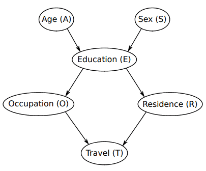
In the previous section we represented the interactions between Age, Sex, Education, Occupation, Residence and Travel using a DAG. To complete the BN modelling the survey, we will now specify a joint probability distribution over these variables. All of them are discrete and defined on a set of nonordered states (called levels in $\mathrm{R}$ ).

Therefore, the natural choice for the joint probability distribution is a multinomial distribution, assigning a probability to each combination of states of the variables in the survey. In the context of $\mathrm{BNs}$, this joint distribution is called the global distribution.

However, using the global distribution directly is difficult: even for small problems, such as that we are considering, the number of parameters involved is very high. In the case of this survey, the parameter set includes the 143 probabilities corresponding to the combinations of the levels of all the variables. Fortunately, we can use the information encoded in the DAG to break down the global distribution into a set of smaller local distributions, one for each variable. Recall that arcs represent direct dependencies: if there is an arc from one variable to another, the latter depends on the former. In other words, variables that are not linked by an arc are conditionally independent. As a result, we can factorise the global distribution as follows:
$$
\operatorname{Pr}(A, S, E, 0, R, T)=\operatorname{Pr}(A) \operatorname{Pr}(S) \operatorname{Pr}(E \mid A, S) \operatorname{Pr}(0 \mid E) \operatorname{Pr}(R \mid E) \operatorname{Pr}(T \mid O, R)
$$
Equation (1.1) provides a formal definition of how the dependencies encoded in the DAG map into the probability space via conditional independence relationships. The absence of cycles in the DAG ensures that the factorisation is well defined. Each variable depends only on its parents; its distribution is univariate and has a (comparatively) small number of parameters. The set of all the local distributions has, overall, fewer parameters than the global distribution. The latter represents a more general model than the former, because it does not make any assumption on the dependencies between the variables. In other words, the factorisation in Equation (1.1) defines a nested model or a submodel of the global distribution.

统计代写|贝叶斯网络代写Bayesian network代考|Learning the DAG Structure: Tests and Scores

In the previous sections we have assumed that the DAG underlying the BN is known. In other words, we rely on prior knowledge on the phenomenon we are modelling to decide which arcs are present in the graph and which are not. However, this is not always possible or desired; the structure of the DAG itself may be the object of our investigation. It is common in genetics and systems biology, for instance, to reconstruct the molecular pathways and networks underlying complex diseases and metabolic processes. An outstanding example of this kind of study can be found in Sachs et al. (2005) and will be explored in Chapter 8. In the context of social sciences, the structure of the DAG may identify which nodes are directly related to the target of the analysis and may therefore be used to improve the process of policy making. For instance, the

DAG of the survey we are using as an example suggests that train fares should be adjusted (to maximise profit) on the basis of Occupation and Residence alone.

Learning the DAG of a $\mathrm{BN}$ is a complex task, for two reasons. First, the space of the possible DAGs is very big; the number of DAGs increases superexponentially as the number of nodes grows. As a result, only a small fraction of its elements can be investigated in a reasonable time. Furthermore, this space is very different from real spaces (e.g., $\mathbb{R}, \mathbb{R}^{2}, \mathbb{R}^{3}$, etc.) in that it is not continuous and has a finite number of elements. Therefore, ad-hoc algorithms are required to explore it. We will investigate the algorithms proposed for this task and their theoretical foundations in Section 6.5. For the moment, we will limit our attention to the two classes of statistical criteria used by those algorithms to evaluate DAGs: conditional independence tests and network schrest.

贝叶斯网络代考

统计代写|贝叶斯网络代写Bayesian network代考| Probabilistic Representation

在上一节中，我们使用 DAG 表示了年龄、性别、教育、职业、居住地和旅行之间的相互作用。为了完成对调查的 BN 建模，我们现在将指定这些变量的联合概率分布。它们都是离散的，并定义在一组无序状态（在R ).

因此，联合概率分布的自然选择是多项分布，为调查中变量的每个状态组合分配一个概率。在上下文中乙ñs，这种联合分布称为全局分布。

然而，直接使用全局分布是困难的：即使对于小问题，例如我们正在考虑的问题，所涉及的参数数量也非常多。在本次调查的情况下，参数集包括对应于所有变量水平组合的 143 个概率。幸运的是，我们可以使用 DAG 中编码的信息将全局分布分解为一组较小的局部分布，每个变量一个。回想一下弧表示直接依赖关系：如果从一个变量到另一个变量存在弧，则后者依赖于前者。换句话说，未通过弧链接的变量是条件独立的。因此，我们可以将全局分布分解如下：

公关⁡(一个,小号,和,0,R,吨)=公关⁡(一个)公关⁡(小号)公关⁡(和∣一个,小号)公关⁡(0∣和)公关⁡(R∣和)公关⁡(吨∣○,R)
等式 (1.1) 提供了 DAG 中编码的依赖关系如何通过条件独立关系映射到概率空间的正式定义。DAG 中没有循环确保了分解是明确定义的。每个变量仅取决于其父项；它的分布是单变量的，并且具有（相对）少量的参数。总体而言，所有局部分布的集合比全局分布具有更少的参数。后者代表了比前者更通用的模型，因为它不对变量之间的依赖关系做出任何假设。换句话说，等式（1.1）中的分解定义了一个嵌套模型或全局分布的子模型。

统计代写|贝叶斯网络代写Bayesian network代考|Learning the DAG Structure: Tests and Scores

在前面的部分中，我们假设 BN 下的 DAG 是已知的。换句话说，我们依赖于我们正在建模的现象的先验知识来确定图中存在哪些弧，哪些不存在。然而，这并不总是可能或不希望的；DAG 本身的结构可能是我们研究的对象。例如，重建复杂疾病和代谢过程的分子途径和网络在遗传学和系统生物学中很常见。此类研究的一个突出例子可以在 Sachs 等人中找到。（2005 年）并将在第 8 章进行探讨。在社会科学的背景下，DAG 的结构可以确定哪些节点与分析目标直接相关，因此可以用于改进政策制定过程。例如，

我们以调查的 DAG 为例，建议仅根据职业和居住地调整火车票价（以最大化利润）。

学习一个 DAG乙ñ是一项复杂的任务，原因有二。首先，可能的 DAG 空间很大；随着节点数量的增加，DAG 的数量呈超指数增长。结果，在合理的时间内只能研究其元素的一小部分。此外，这个空间与真实空间非常不同（例如，R,R2,R3等），因为它不是连续的并且具有有限数量的元素。因此，需要专门的算法来探索它。我们将在 6.5 节研究为此任务提出的算法及其理论基础。目前，我们将把注意力限制在这些算法用来评估 DAG 的两类统计标准上：条件独立性测试和网络 schrest。

统计代写请认准statistics-lab™. statistics-lab™为您的留学生涯保驾护航。

金融工程代写

金融工程是使用数学技术来解决金融问题。金融工程使用计算机科学、统计学、经济学和应用数学领域的工具和知识来解决当前的金融问题，以及设计新的和创新的金融产品。

非参数统计代写

非参数统计指的是一种统计方法，其中不假设数据来自于由少数参数决定的规定模型；这种模型的例子包括正态分布模型和线性回归模型。

广义线性模型代考

广义线性模型（GLM）归属统计学领域，是一种应用灵活的线性回归模型。该模型允许因变量的偏差分布有除了正态分布之外的其它分布。

术语 广义线性模型（GLM）通常是指给定连续和/或分类预测因素的连续响应变量的常规线性回归模型。它包括多元线性回归，以及方差分析和方差分析（仅含固定效应）。

有限元方法代写

有限元方法（FEM）是一种流行的方法，用于数值解决工程和数学建模中出现的微分方程。典型的问题领域包括结构分析、传热、流体流动、质量运输和电磁势等传统领域。

有限元是一种通用的数值方法，用于解决两个或三个空间变量的偏微分方程（即一些边界值问题）。为了解决一个问题，有限元将一个大系统细分为更小、更简单的部分，称为有限元。这是通过在空间维度上的特定空间离散化来实现的，它是通过构建对象的网格来实现的：用于求解的数值域，它有有限数量的点。边界值问题的有限元方法表述最终导致一个代数方程组。该方法在域上对未知函数进行逼近。[1] 然后将模拟这些有限元的简单方程组合成一个更大的方程系统，以模拟整个问题。然后，有限元通过变化微积分使相关的误差函数最小化来逼近一个解决方案。

tatistics-lab作为专业的留学生服务机构，多年来已为美国、英国、加拿大、澳洲等留学热门地的学生提供专业的学术服务，包括但不限于Essay代写，Assignment代写，Dissertation代写，Report代写，小组作业代写，Proposal代写，Paper代写，Presentation代写，计算机作业代写，论文修改和润色，网课代做，exam代考等等。写作范围涵盖高中，本科，研究生等海外留学全阶段，辐射金融，经济学，会计学，审计学，管理学等全球99%专业科目。写作团队既有专业英语母语作者，也有海外名校硕博留学生，每位写作老师都拥有过硬的语言能力，专业的学科背景和学术写作经验。我们承诺100%原创，100%专业，100%准时，100%满意。

随机分析代写

随机微积分是数学的一个分支，对随机过程进行操作。它允许为随机过程的积分定义一个关于随机过程的一致的积分理论。这个领域是由日本数学家伊藤清在第二次世界大战期间创建并开始的。

时间序列分析代写

随机过程，是依赖于参数的一组随机变量的全体，参数通常是时间。 随机变量是随机现象的数量表现，其时间序列是一组按照时间发生先后顺序进行排列的数据点序列。通常一组时间序列的时间间隔为一恒定值（如1秒，5分钟，12小时，7天，1年），因此时间序列可以作为离散时间数据进行分析处理。研究时间序列数据的意义在于现实中，往往需要研究某个事物其随时间发展变化的规律。这就需要通过研究该事物过去发展的历史记录，以得到其自身发展的规律。

回归分析代写

多元回归分析渐进（Multiple Regression Analysis Asymptotics）属于计量经济学领域，主要是一种数学上的统计分析方法，可以分析复杂情况下各影响因素的数学关系，在自然科学、社会和经济学等多个领域内应用广泛。

MATLAB代写

MATLAB 是一种用于技术计算的高性能语言。它将计算、可视化和编程集成在一个易于使用的环境中，其中问题和解决方案以熟悉的数学符号表示。典型用途包括：数学和计算算法开发建模、仿真和原型制作数据分析、探索和可视化科学和工程图形应用程序开发，包括图形用户界面构建MATLAB 是一个交互式系统，其基本数据元素是一个不需要维度的数组。这使您可以解决许多技术计算问题，尤其是那些具有矩阵和向量公式的问题，而只需用 C 或 Fortran 等标量非交互式语言编写程序所需的时间的一小部分。MATLAB 名称代表矩阵实验室。MATLAB 最初的编写目的是提供对由 LINPACK 和 EISPACK 项目开发的矩阵软件的轻松访问，这两个项目共同代表了矩阵计算软件的最新技术。MATLAB 经过多年的发展，得到了许多用户的投入。在大学环境中，它是数学、工程和科学入门和高级课程的标准教学工具。在工业领域，MATLAB 是高效研究、开发和分析的首选工具。MATLAB 具有一系列称为工具箱的特定于应用程序的解决方案。对于大多数 MATLAB 用户来说非常重要，工具箱允许您学习和应用专业技术。工具箱是 MATLAB 函数（M 文件）的综合集合，可扩展 MATLAB 环境以解决特定类别的问题。可用工具箱的领域包括信号处理、控制系统、神经网络、模糊逻辑、小波、仿真等。

R语言代写	问卷设计与分析代写
PYTHON代写	回归分析与线性模型代写
MATLAB代写	方差分析与试验设计代写
STATA代写	机器学习/统计学习代写
SPSS代写	计量经济学代写
EVIEWS代写	时间序列分析代写
EXCEL代写	深度学习代写
SQL代写	各种数据建模与可视化代写

如果你也在 怎样代写贝叶斯网络Bayesian network这个学科遇到相关的难题，请随时右上角联系我们的24/7代写客服。

贝叶斯网络（BN）是一种表示不确定领域知识的概率图形模型，其中每个节点对应一个随机变量，每条边代表相应随机变量的条件概率。

statistics-lab™ 为您的留学生涯保驾护航 在代写贝叶斯网络Bayesian network方面已经树立了自己的口碑, 保证靠谱, 高质且原创的统计Statistics代写服务。我们的专家在代写贝叶斯网络Bayesian network代写方面经验极为丰富，各种代写贝叶斯网络Bayesian network相关的作业也就用不着说。

我们提供的贝叶斯网络Bayesian network及其相关学科的代写，服务范围广, 其中包括但不限于:

• Statistical Inference 统计推断
• Statistical Computing 统计计算
• Advanced Probability Theory 高等概率论
• Advanced Mathematical Statistics 高等数理统计学
• (Generalized) Linear Models 广义线性模型
• Statistical Machine Learning 统计机器学习
• Longitudinal Data Analysis 纵向数据分析
• Foundations of Data Science 数据科学基础

统计代写|贝叶斯网络代写Bayesian network代考| Train-Use Survey

Consider a simple, hypothetical survey whose aim is to investigate the usage patterns of different means of transport, with a focus on cars and trains. Such surveys are used to assess customer satisfaction across different social groups, to evaluate public policies and to improve urban planning. Some real-world examples can be found, for instance, in Kenett et al. (2012).

In our current example we will examine, for each individual, the following six discrete variables (labels used in computations and figures are reported in parenthesis):

• Age (A): the age, recorded as young (young) for individuals below 30 years old, adult (adult) for individuals between 30 and 60 years old, and old (old) for people older than 60 .
• Sex (S): the biological sex, recorded as male (M) or female (F).
• Education (E): the highest level of education or training successfully completed, recorded as up to high school (high) or university degree (uni).
• Occupation (0): whether the individual is an employee (emp) or a selfemployed (self) worker.
• Residence (R): the size of the city the individual lives in, recorded as either small (small) or big (big).
• Travel (T): the means of transport favoured by the individual, recorded either as car (car), train (train) or other (other).
• In the scope of this survey, each variable falls into one of three groups. Age and Sex are demographic indicators. In other words, they are intrinsic characteristics of the individual; they may result in different patterns of behaviour but are not influenced by the individual himself. On the other hand, the opposite is true for Education, Occupation and Residence. These variables are socioeconomic indicators and describe the individual’s position in society. Therefore, they provide a rough description of the individual’s expected lifestyle; for example, they may characterise his spending habits and his work schedule. The last variable, Travel, is the target of the survey, the quantity of interest whose behaviour is under investigation.

统计代写|贝叶斯网络代写Bayesian network代考|Graphical Representation

The nature of the variables recorded in the survey, and more in general of the three categories they belong to, suggests how they may be related with each other. Some of these relationships will be direct, while others will be mediated by one or more variables (indirect).

Both kinds of relationships can be represented effectively and intuitively by means of a directed graph, which is one of the two fundamental entities characterising a BN. Each node in the graph corresponds to one of the variables in the survey. In fact, they are usually referred to interchangeably in the literature. Therefore, the graph produced from this example will contain six nodes, labelled after the variabless (A, S, E, $0, R$ and $T$ ). Direct dependence relationships are represented as arcs between pairs of variables (e.g., $A \rightarrow E$ means that $E$ depends on A). The node at the tail of the arc is called the parent, while that at the head (where the arrow is) is called the child. Indirect dependence relationships are not explicitly represented. However, they can be read from the graph as sequences of arcs leading from one variable to the other through one or more mediating variables (e.g., the combination of $A \rightarrow E$ and $E \rightarrow R$ means that $R$ depends on $A$ through $E$ ). Such sequences of arcs are said to form a path leading from one variable to the other; these two variables must be distinct. Paths of the form $\mathrm{A} \rightarrow \ldots \rightarrow \mathrm{A}$, which are known as cycles, are not allowed in the graph. For this reason, the graphs used in BNs are called directed acyclic graphs (DAGs).

Note, however, that some caution must be exercised in interpreting both direct and indirect dependencies. The presence of arrows or arcs seems to imply, at an intuitive level, that for each arc one variable should be interpreted as a cause and the other as an effect (e.g., $A \rightarrow E$ means that A causes $E$ ). This interpretation, which is called causal, is difficult to justify in most situations: for this reason, in general we speak about dependence relationships instead of causal effects. The assumptions required for causal BN modelling will be discussed in Section 6.7.

贝叶斯网络代考

统计代写|贝叶斯网络代写Bayesian network代考| Train-Use Survey

考虑一个简单的假设性调查，其目的是调查不同交通工具的使用模式，重点是汽车和火车。此类调查用于评估不同社会群体的客户满意度、评估公共政策和改进城市规划。例如，可以在 Kenett 等人中找到一些现实世界的例子。（2012）。

在我们当前的示例中，我们将为每个人检查以下六个离散变量（计算中使用的标签和数字在括号中报告）：

• 年龄（A）：年龄，30岁以下记录为年轻（young），30-60岁记录为成人（adult），60岁以上记录为老人（old）。
• 性别（S）：生理性别，记为男性（M）或女性（F）。
• 教育（E）：成功完成的最高教育或培训水平，记录为高中（high）或大学学位（uni）。
• 职业（0）：个人是雇员（emp）还是个体经营者（self）。
• 居住地（R）：个人居住城市的大小，记为小（小）或大（大）。
• 旅行（T）：个人喜欢的交通工具，记为汽车（car）、火车（train）或其他（other）。
• 在本次调查的范围内，每个变量都属于三组之一。年龄和性别是人口统计指标。换句话说，它们是个体的内在特征；它们可能导致不同的行为模式，但不受个人本人的影响。另一方面，教育、职业和居住则相反。这些变量是社会经济指标，描述了个人在社会中的地位。因此，它们提供了个人预期生活方式的粗略描述；例如，它们可以描述他的消费习惯和工作日程。最后一个变量 Travel 是调查的目标，即正在调查其行为的兴趣数量。

统计代写|贝叶斯网络代写Bayesian network代考|Graphical Representation

调查中记录的变量的性质，以及它们所属的三个类别的更一般性，表明它们可能如何相互关联。其中一些关系将是直接的，而其他关系将由一个或多个变量（间接）介导。

这两种关系都可以通过有向图来有效和直观地表示，有向图是表征 BN 的两个基本实体之一。图中的每个节点对应于调查中的一个变量。事实上，它们在文献中通常可以互换使用。因此，此示例生成的图将包含六个节点，在变量（A、S、E、0,R和吨）。直接依赖关系表示为变量对之间的弧（例如，一个→和意思是和取决于 A)。弧尾部的节点称为父节点，而弧头（箭头所在的位置）的节点称为子节点。间接依赖关系没有明确表示。但是，它们可以从图中读取为通过一个或多个中介变量从一个变量到另一个变量的弧序列（例如，一个→和和和→R意思是R取决于一个通过和）。据说这样的弧序列形成了从一个变量到另一个变量的路径。这两个变量必须是不同的。表格路径一个→…→一个，称为循环，在图中是不允许的。因此，BN 中使用的图称为有向无环图 (DAG)。

但是请注意，在解释直接和间接依赖关系时必须小心谨慎。箭头或弧线的存在似乎暗示，在直观的层面上，对于每条弧线，一个变量应该被解释为原因，而另一个变量应该被解释为结果（例如，一个→和意味着 A 导致和）。这种被称为因果关系的解释在大多数情况下很难证明是正确的：因此，通常我们谈论的是依赖关系而不是因果关系。因果 BN 建模所需的假设将在第 6.7 节中讨论。

统计代写请认准statistics-lab™. statistics-lab™为您的留学生涯保驾护航。

金融工程代写

金融工程是使用数学技术来解决金融问题。金融工程使用计算机科学、统计学、经济学和应用数学领域的工具和知识来解决当前的金融问题，以及设计新的和创新的金融产品。

非参数统计代写

非参数统计指的是一种统计方法，其中不假设数据来自于由少数参数决定的规定模型；这种模型的例子包括正态分布模型和线性回归模型。

广义线性模型代考

广义线性模型（GLM）归属统计学领域，是一种应用灵活的线性回归模型。该模型允许因变量的偏差分布有除了正态分布之外的其它分布。

术语 广义线性模型（GLM）通常是指给定连续和/或分类预测因素的连续响应变量的常规线性回归模型。它包括多元线性回归，以及方差分析和方差分析（仅含固定效应）。

有限元方法代写

有限元方法（FEM）是一种流行的方法，用于数值解决工程和数学建模中出现的微分方程。典型的问题领域包括结构分析、传热、流体流动、质量运输和电磁势等传统领域。

有限元是一种通用的数值方法，用于解决两个或三个空间变量的偏微分方程（即一些边界值问题）。为了解决一个问题，有限元将一个大系统细分为更小、更简单的部分，称为有限元。这是通过在空间维度上的特定空间离散化来实现的，它是通过构建对象的网格来实现的：用于求解的数值域，它有有限数量的点。边界值问题的有限元方法表述最终导致一个代数方程组。该方法在域上对未知函数进行逼近。[1] 然后将模拟这些有限元的简单方程组合成一个更大的方程系统，以模拟整个问题。然后，有限元通过变化微积分使相关的误差函数最小化来逼近一个解决方案。

tatistics-lab作为专业的留学生服务机构，多年来已为美国、英国、加拿大、澳洲等留学热门地的学生提供专业的学术服务，包括但不限于Essay代写，Assignment代写，Dissertation代写，Report代写，小组作业代写，Proposal代写，Paper代写，Presentation代写，计算机作业代写，论文修改和润色，网课代做，exam代考等等。写作范围涵盖高中，本科，研究生等海外留学全阶段，辐射金融，经济学，会计学，审计学，管理学等全球99%专业科目。写作团队既有专业英语母语作者，也有海外名校硕博留学生，每位写作老师都拥有过硬的语言能力，专业的学科背景和学术写作经验。我们承诺100%原创，100%专业，100%准时，100%满意。

随机分析代写

随机微积分是数学的一个分支，对随机过程进行操作。它允许为随机过程的积分定义一个关于随机过程的一致的积分理论。这个领域是由日本数学家伊藤清在第二次世界大战期间创建并开始的。

时间序列分析代写

随机过程，是依赖于参数的一组随机变量的全体，参数通常是时间。 随机变量是随机现象的数量表现，其时间序列是一组按照时间发生先后顺序进行排列的数据点序列。通常一组时间序列的时间间隔为一恒定值（如1秒，5分钟，12小时，7天，1年），因此时间序列可以作为离散时间数据进行分析处理。研究时间序列数据的意义在于现实中，往往需要研究某个事物其随时间发展变化的规律。这就需要通过研究该事物过去发展的历史记录，以得到其自身发展的规律。

回归分析代写

多元回归分析渐进（Multiple Regression Analysis Asymptotics）属于计量经济学领域，主要是一种数学上的统计分析方法，可以分析复杂情况下各影响因素的数学关系，在自然科学、社会和经济学等多个领域内应用广泛。

MATLAB代写

MATLAB 是一种用于技术计算的高性能语言。它将计算、可视化和编程集成在一个易于使用的环境中，其中问题和解决方案以熟悉的数学符号表示。典型用途包括：数学和计算算法开发建模、仿真和原型制作数据分析、探索和可视化科学和工程图形应用程序开发，包括图形用户界面构建MATLAB 是一个交互式系统，其基本数据元素是一个不需要维度的数组。这使您可以解决许多技术计算问题，尤其是那些具有矩阵和向量公式的问题，而只需用 C 或 Fortran 等标量非交互式语言编写程序所需的时间的一小部分。MATLAB 名称代表矩阵实验室。MATLAB 最初的编写目的是提供对由 LINPACK 和 EISPACK 项目开发的矩阵软件的轻松访问，这两个项目共同代表了矩阵计算软件的最新技术。MATLAB 经过多年的发展，得到了许多用户的投入。在大学环境中，它是数学、工程和科学入门和高级课程的标准教学工具。在工业领域，MATLAB 是高效研究、开发和分析的首选工具。MATLAB 具有一系列称为工具箱的特定于应用程序的解决方案。对于大多数 MATLAB 用户来说非常重要，工具箱允许您学习和应用专业技术。工具箱是 MATLAB 函数（M 文件）的综合集合，可扩展 MATLAB 环境以解决特定类别的问题。可用工具箱的领域包括信号处理、控制系统、神经网络、模糊逻辑、小波、仿真等。

R语言代写	问卷设计与分析代写
PYTHON代写	回归分析与线性模型代写
MATLAB代写	方差分析与试验设计代写
STATA代写	机器学习/统计学习代写
SPSS代写	计量经济学代写
EVIEWS代写	时间序列分析代写
EXCEL代写	深度学习代写
SQL代写	各种数据建模与可视化代写