标签： KMA322

数学代写|泛函分析作业代写Functional Analysis代考|Scalar (Inner) Product, Representation Theorem in Finite-Dimensional Spaces

Posted on 2023年6月15日2023年6月15日 by statistics-lab

如果你也在怎样代写泛函分析functional analysis MATH4010这个学科遇到相关的难题，请随时右上角联系我们的24/7代写客服。泛函分析functional analysis是数学分析的一个分支，其核心是研究具有某种极限相关结构（如内积、规范、拓扑等）的向量空间以及定义在这些空间上并在适当意义上尊重这些结构的线性函数。

泛函分析functional analysis是数学分析的一个分支，其核心是研究具有某种极限相关结构（如内积、规范、拓扑等）的向量空间以及定义在这些空间上并在适当意义上尊重这些结构的线性函数。函数分析的历史根源在于对函数空间的研究，以及对函数变换属性的表述，例如将傅里叶变换作为定义函数空间之间的连续、单元等算子的变换。这一观点对微分和积分方程的研究特别有用。

statistics-lab™ 为您的留学生涯保驾护航在代写泛函分析Functional Analysis方面已经树立了自己的口碑, 保证靠谱, 高质且原创的统计Statistics代写服务。我们的专家在代写泛函分析Functional Analysis代写方面经验极为丰富，各种代写泛函分析Functional Analysis相关的作业也就用不着说。

数学代写|泛函分析作业代写Functional Analysis代考|Scalar (Inner) Product, Representation Theorem in Finite-Dimensional Spaces

In this section we shall deal with a generalization of the “dot-product” or inner product of two vectors.
Scalar (Inner) Product. Let $V$ be a complex vector space. A complex valued function from $V \times V$ into $\mathbb{C}$ that associates with each pair $\boldsymbol{u}, \boldsymbol{v}$ of vectors in $V$ a scalar, denoted $(\boldsymbol{u}, \boldsymbol{v})_V$ or shortly $(\boldsymbol{u}, \boldsymbol{v})$ if no confusion occurs, is called a scalar (inner) product on $V$ if and only if
(i) $\left(\alpha_1 \boldsymbol{u}_1+\alpha_2 \boldsymbol{u}_2, \boldsymbol{v}\right)=\alpha_1\left(\boldsymbol{u}_1, \boldsymbol{v}\right)+\alpha_2\left(\boldsymbol{u}_2, \boldsymbol{v}\right)$, i.e., $(\boldsymbol{u}, \boldsymbol{v})$ is linear with respect to $\boldsymbol{u}$.
(ii) $(\boldsymbol{u}, \boldsymbol{v})=\overline{(\boldsymbol{v}, \boldsymbol{u})}$, where $\overline{(\boldsymbol{v}, \boldsymbol{u})}$ denotes the complex conjugate of $(\boldsymbol{v}, \boldsymbol{v})$ (antisymmetry).
(iii) $(\boldsymbol{u}, \boldsymbol{u})$ is positively defined, i.e., $(\boldsymbol{u}, \boldsymbol{u}) \geq 0$ and $(\boldsymbol{u}, \boldsymbol{u})=0$ implies $\boldsymbol{u}=\mathbf{0}$.
Let us note that due to antisymmetry $(\boldsymbol{u}, \boldsymbol{u})$ is a real number and therefore it makes sense to speak about positive definiteness. The first two conditions imply that $(\boldsymbol{u}, \boldsymbol{v})$ is antilinear with respect to the second variable
$$
\left(\boldsymbol{u}, \beta_1 \boldsymbol{v}_1+\beta_2 \boldsymbol{v}_2\right)=\bar{\beta}_1\left(\boldsymbol{u}, \boldsymbol{v}_1\right)+\bar{\beta}_2\left(\boldsymbol{u}, \boldsymbol{v}_2\right)
$$
In most of the developments to follow, we shall deal with real vector spaces only. Then property (ii) becomes one of symmetry
(ii) $(\boldsymbol{u}, \boldsymbol{v})=(\boldsymbol{v}, \boldsymbol{u})$
and the inner product becomes a bilinear functional.

数学代写|泛函分析作业代写Functional Analysis代考|Basis and Cobasis, Adjoint of a Transformation, Contra- and Covariant Components of Tensors

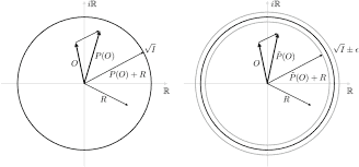
The Representation Theorem with the Riesz map allows us, in the case of a finite-dimensional inner product space $V$, to identify the dual $V^$ with the original space $V$. Consequently, every notion which has been defined for dual space $V^$ can now be reinterpreted in the context of the inner product space.

Through this section $V$ will denote a finite-dimensional vector space with an inner product $(\cdot, \cdot)$ and the corresponding Riesz map
$$
R: V \ni \boldsymbol{u} \rightarrow \boldsymbol{u}^=(\cdot, \boldsymbol{u}) \in V^
$$
Cobasis. Let $\boldsymbol{e}i, i=1, \ldots, n$ be a basis and $\boldsymbol{e}_j^, j=1, \ldots, n$ its dual basis. Consider vectors $$ e^j=R^{-1} e_j^
$$
According to the definition of the Riesz map, we have
$$
\left(\boldsymbol{e}_i, \boldsymbol{e}^j\right)=\overline{\left(\boldsymbol{e}^j, \boldsymbol{e}_i\right)}=\overline{\left(R^{-1} \boldsymbol{e}_j^, \boldsymbol{e}_i\right)}=\left\langle\boldsymbol{e}_j^, \boldsymbol{e}_i\right\rangle=\delta{i j}
$$
COROLLARY 2.15.1
For a given basis $e_i, i=1, \ldots, n$, there exists a unique basis $\boldsymbol{e}^j$ (called cobasis) such that
$$
\left(\boldsymbol{e}i, \boldsymbol{e}^j\right)=\delta{i j}
$$

Orthogonal Complements. Let $U$ be a subspace of $V$ and $U^{\perp}$ denote its orthogonal complement in $V^*$. The inverse image of $U^{\perp}$ by the Riesz map
$$
R^{-1}\left(U^{\perp}\right)
$$
denoted by the same symbol $U^{\perp}$ will also be called the orthogonal complement (in $V$ ) of subspace $U$. Let $\boldsymbol{u} \in U, \boldsymbol{v} \in U^{\perp}$. We have
$$
(\boldsymbol{u}, \boldsymbol{v})=\langle R \boldsymbol{v}, \boldsymbol{u}\rangle=0
$$
Thus the orthogonal complement can be expressed in the form
$$
U^{\perp}={\boldsymbol{v} \in \boldsymbol{V}:(\boldsymbol{u}, \boldsymbol{v})=0 \text { for every } \boldsymbol{u} \in U}
$$

泛函分析代写

数学代写|泛函分析作业代写Functional Analysis代考|Scalar (Inner) Product, Representation Theorem in Finite-Dimensional Spaces

在本节中，我们将处理“点积”或两个向量的内积的推广。
标量(内)积。设$V$是一个复向量空间。从$V \times V$到$\mathbb{C}$的复值函数与$V$中的每对$\boldsymbol{u}, \boldsymbol{v}$向量关联一个标量，如果没有混淆，表示为$(\boldsymbol{u}, \boldsymbol{v})_V$或简称为$(\boldsymbol{u}, \boldsymbol{v})$，在$V$上称为标量(内)积，当且仅当
(i) $\left(\alpha_1 \boldsymbol{u}_1+\alpha_2 \boldsymbol{u}_2, \boldsymbol{v}\right)=\alpha_1\left(\boldsymbol{u}_1, \boldsymbol{v}\right)+\alpha_2\left(\boldsymbol{u}_2, \boldsymbol{v}\right)$，即$(\boldsymbol{u}, \boldsymbol{v})$相对于$\boldsymbol{u}$是线性的。
(ii) $(\boldsymbol{u}, \boldsymbol{v})=\overline{(\boldsymbol{v}, \boldsymbol{u})}$，其中$\overline{(\boldsymbol{v}, \boldsymbol{u})}$表示$(\boldsymbol{v}, \boldsymbol{v})$(反对称)的复共轭。
(iii) $(\boldsymbol{u}, \boldsymbol{u})$是积极定义的，即$(\boldsymbol{u}, \boldsymbol{u}) \geq 0$和$(\boldsymbol{u}, \boldsymbol{u})=0$意味着$\boldsymbol{u}=\mathbf{0}$。
让我们注意到，由于不对称$(\boldsymbol{u}, \boldsymbol{u})$是一个实数，因此谈论正确定性是有意义的。前两个条件意味着$(\boldsymbol{u}, \boldsymbol{v})$对第二个变量是反线性的
$$
\left(\boldsymbol{u}, \beta_1 \boldsymbol{v}_1+\beta_2 \boldsymbol{v}_2\right)=\bar{\beta}_1\left(\boldsymbol{u}, \boldsymbol{v}_1\right)+\bar{\beta}_2\left(\boldsymbol{u}, \boldsymbol{v}_2\right)
$$
在接下来的大多数发展中，我们将只处理实向量空间。那么性质(ii)就变成了对称性质
(ii) $(\boldsymbol{u}, \boldsymbol{v})=(\boldsymbol{v}, \boldsymbol{u})$
内积变成了双线性泛函。

数学代写|泛函分析作业代写Functional Analysis代考|Basis and Cobasis, Adjoint of a Transformation, Contra- and Covariant Components of Tensors

在有限维内积空间$V$的情况下，Riesz映射的表示定理允许我们识别对偶$V^$与原始空间$V$。因此，在对偶空间$V^$中定义的每一个概念现在都可以在内积空间的背景下重新解释。

通过本节，$V$将表示具有内积$(\cdot, \cdot)$和相应Riesz映射的有限维向量空间
$$
R: V \ni \boldsymbol{u} \rightarrow \boldsymbol{u}^=(\cdot, \boldsymbol{u}) \in V^
$$
共基。设$\boldsymbol{e}i, i=1, \ldots, n$为基，$\boldsymbol{e}_j^, j=1, \ldots, n$为双基。考虑向量$$ e^j=R^{-1} e_j^
$$
根据Riesz地图的定义，我们有
$$
\left(\boldsymbol{e}_i, \boldsymbol{e}^j\right)=\overline{\left(\boldsymbol{e}^j, \boldsymbol{e}_i\right)}=\overline{\left(R^{-1} \boldsymbol{e}_j^, \boldsymbol{e}_i\right)}=\left\langle\boldsymbol{e}_j^, \boldsymbol{e}_i\right\rangle=\delta{i j}
$$
推论2.15.1
对于给定的基$e_i, i=1, \ldots, n$，存在唯一的基$\boldsymbol{e}^j$(称为共基)，使得
$$
\left(\boldsymbol{e}i, \boldsymbol{e}^j\right)=\delta{i j}
$$

正交补。设$U$是$V$的一个子空间，$U^{\perp}$表示它在$V^*$中的正交补。Riesz地图上$U^{\perp}$的逆图像
$$
R^{-1}\left(U^{\perp}\right)
$$
用同样的符号表示$U^{\perp}$也称为子空间$U$的正交补(在$V$中)。让$\boldsymbol{u} \in U, \boldsymbol{v} \in U^{\perp}$。我们有
$$
(\boldsymbol{u}, \boldsymbol{v})=\langle R \boldsymbol{v}, \boldsymbol{u}\rangle=0
$$
因此，正交补可以表示为
$$
U^{\perp}={\boldsymbol{v} \in \boldsymbol{V}:(\boldsymbol{u}, \boldsymbol{v})=0 \text { for every } \boldsymbol{u} \in U}
$$

数学代写|泛函分析作业代写Functional Analysis代考请认准statistics-lab™

统计代写请认准statistics-lab™. statistics-lab™为您的留学生涯保驾护航。

金融工程代写

金融工程是使用数学技术来解决金融问题。金融工程使用计算机科学、统计学、经济学和应用数学领域的工具和知识来解决当前的金融问题，以及设计新的和创新的金融产品。

非参数统计代写

非参数统计指的是一种统计方法，其中不假设数据来自于由少数参数决定的规定模型；这种模型的例子包括正态分布模型和线性回归模型。

广义线性模型代考

广义线性模型（GLM）归属统计学领域，是一种应用灵活的线性回归模型。该模型允许因变量的偏差分布有除了正态分布之外的其它分布。

术语广义线性模型（GLM）通常是指给定连续和/或分类预测因素的连续响应变量的常规线性回归模型。它包括多元线性回归，以及方差分析和方差分析（仅含固定效应）。

有限元方法代写

有限元方法（FEM）是一种流行的方法，用于数值解决工程和数学建模中出现的微分方程。典型的问题领域包括结构分析、传热、流体流动、质量运输和电磁势等传统领域。

有限元是一种通用的数值方法，用于解决两个或三个空间变量的偏微分方程（即一些边界值问题）。为了解决一个问题，有限元将一个大系统细分为更小、更简单的部分，称为有限元。这是通过在空间维度上的特定空间离散化来实现的，它是通过构建对象的网格来实现的：用于求解的数值域，它有有限数量的点。边界值问题的有限元方法表述最终导致一个代数方程组。该方法在域上对未知函数进行逼近。[1] 然后将模拟这些有限元的简单方程组合成一个更大的方程系统，以模拟整个问题。然后，有限元通过变化微积分使相关的误差函数最小化来逼近一个解决方案。

tatistics-lab作为专业的留学生服务机构，多年来已为美国、英国、加拿大、澳洲等留学热门地的学生提供专业的学术服务，包括但不限于Essay代写，Assignment代写，Dissertation代写，Report代写，小组作业代写，Proposal代写，Paper代写，Presentation代写，计算机作业代写，论文修改和润色，网课代做，exam代考等等。写作范围涵盖高中，本科，研究生等海外留学全阶段，辐射金融，经济学，会计学，审计学，管理学等全球99%专业科目。写作团队既有专业英语母语作者，也有海外名校硕博留学生，每位写作老师都拥有过硬的语言能力，专业的学科背景和学术写作经验。我们承诺100%原创，100%专业，100%准时，100%满意。

随机分析代写

随机微积分是数学的一个分支，对随机过程进行操作。它允许为随机过程的积分定义一个关于随机过程的一致的积分理论。这个领域是由日本数学家伊藤清在第二次世界大战期间创建并开始的。

时间序列分析代写

随机过程，是依赖于参数的一组随机变量的全体，参数通常是时间。随机变量是随机现象的数量表现，其时间序列是一组按照时间发生先后顺序进行排列的数据点序列。通常一组时间序列的时间间隔为一恒定值（如1秒，5分钟，12小时，7天，1年），因此时间序列可以作为离散时间数据进行分析处理。研究时间序列数据的意义在于现实中，往往需要研究某个事物其随时间发展变化的规律。这就需要通过研究该事物过去发展的历史记录，以得到其自身发展的规律。

回归分析代写

多元回归分析渐进（Multiple Regression Analysis Asymptotics）属于计量经济学领域，主要是一种数学上的统计分析方法，可以分析复杂情况下各影响因素的数学关系，在自然科学、社会和经济学等多个领域内应用广泛。

MATLAB代写

MATLAB 是一种用于技术计算的高性能语言。它将计算、可视化和编程集成在一个易于使用的环境中，其中问题和解决方案以熟悉的数学符号表示。典型用途包括：数学和计算算法开发建模、仿真和原型制作数据分析、探索和可视化科学和工程图形应用程序开发，包括图形用户界面构建MATLAB 是一个交互式系统，其基本数据元素是一个不需要维度的数组。这使您可以解决许多技术计算问题，尤其是那些具有矩阵和向量公式的问题，而只需用 C 或 Fortran 等标量非交互式语言编写程序所需的时间的一小部分。MATLAB 名称代表矩阵实验室。MATLAB 最初的编写目的是提供对由 LINPACK 和 EISPACK 项目开发的矩阵软件的轻松访问，这两个项目共同代表了矩阵计算软件的最新技术。MATLAB 经过多年的发展，得到了许多用户的投入。在大学环境中，它是数学、工程和科学入门和高级课程的标准教学工具。在工业领域，MATLAB 是高效研究、开发和分析的首选工具。MATLAB 具有一系列称为工具箱的特定于应用程序的解决方案。对于大多数 MATLAB 用户来说非常重要，工具箱允许您学习和应用专业技术。工具箱是 MATLAB 函数（M 文件）的综合集合，可扩展 MATLAB 环境以解决特定类别的问题。可用工具箱的领域包括信号处理、控制系统、神经网络、模糊逻辑、小波、仿真等。

R语言代写	问卷设计与分析代写
PYTHON代写	回归分析与线性模型代写
MATLAB代写	方差分析与试验设计代写
STATA代写	机器学习/统计学习代写
SPSS代写	计量经济学代写
EVIEWS代写	时间序列分析代写
EXCEL代写	深度学习代写
SQL代写	各种数据建模与可视化代写

数学代写|泛函分析作业代写Functional Analysis代考|Transpose of a Linear Transformation

Posted on 2023年5月29日2023年5月29日 by statistics-lab

如果你也在怎样代写泛函分析Functional Analysis这个学科遇到相关的难题，请随时右上角联系我们的24/7代写客服。

泛函分析，数学分析的分支，处理函数，或函数的函数。它作为一个独立的领域出现在20世纪，当时人们意识到不同的数学过程，从算术到微积分程序，表现出非常相似的特性。

我们提供的泛函分析Functional Analysis及其相关学科的代写，服务范围广, 其中包括但不限于:

Statistical Inference 统计推断
Statistical Computing 统计计算
Advanced Probability Theory 高等概率论
Advanced Mathematical Statistics 高等数理统计学
(Generalized) Linear Models 广义线性模型
Statistical Machine Learning 统计机器学习
Longitudinal Data Analysis 纵向数据分析
Foundations of Data Science 数据科学基础

数学代写|泛函分析作业代写Functional Analysis代考|Transpose of a Linear Transformation

Transpose of a Linear Transformation. Let $V$ and $W$ be two vector spaces over the same field $\mathbb{F}$ and $T$ denote an arbitrary linear transformation from $V$ into $W$. Denoting by $W^$ and $V^$ algebraic duals to $W$ and $V$, respectively, we introduce a new transformation $T^T$ from the algebraic dual $W^$ into algebraic dual $V^$ defined as follows:
$$
T^T: W^* \rightarrow V^, \quad T^T\left(\boldsymbol{w}^\right)=\boldsymbol{w}^* \circ T
$$
Transformation $T^T$ is well defined, i.e., composition $\boldsymbol{w}^* \circ T$ defines (due to linearity of both $T$ and functional $\boldsymbol{w}^$ ) a linear functional on $V . T^T$ is also linear. Transformation $T^T$ is called the transpose of the linear transformation $T$. Using the duality pairing notation we may express the definition of the transpose in the equivalent way: $$ \left\langle T^T \boldsymbol{w}^, \boldsymbol{v}\right\rangle=\left\langle\boldsymbol{w}^, T \boldsymbol{v}\right\rangle \quad \forall \boldsymbol{v} \in V, \boldsymbol{w}^ \in W
$$
Let us note that the transpose $T^T$ acts in the opposite direction to $T$; it maps dual $W^$ into dual $V^$. We may illustrate this by the following simple diagram:
$$
\begin{aligned}
& V \stackrel{T}{\longrightarrow} W \
& V^* \stackrel{T^T}{\longleftarrow} W^* \
&
\end{aligned}
$$

数学代写|泛函分析作业代写Functional Analysis代考|Tensor Products, Covariant and Contravariant Tensors

Let $A$ and $B$ be two arbitrary sets. Given two functionals $f$ and $g$ defined on $A$ and $B$, respectively, we can define a new functional on the Cartesian product $A \times B$, called the product of $f$ and $g$, as
$$
A \times B \ni(x, y) \rightarrow f(x) g(y) \in \mathbb{R}(\boldsymbol{C})
$$

In the case of vector spaces and linear functionals, this simple construction leads to some very important algebraic results.

Tensor Product of Linear Functionals. Given two vector spaces $X$ and $Y$ with their duals $X^, Y^$, we define the tensor product of two functions as
$$
\left(\boldsymbol{x}^* \otimes \boldsymbol{y}^\right)(\boldsymbol{x}, \boldsymbol{y})=\boldsymbol{x}^(\boldsymbol{x}) \boldsymbol{y}^(\boldsymbol{y}) \quad \text { for } \boldsymbol{x} \in X, \boldsymbol{y} \in Y $$ It is easy to see that the tensor product $\boldsymbol{x}^ \otimes \boldsymbol{y}^$ is a bilinear functional on $X \times Y$ and therefore the tensor product can be considered as an operation from the Cartesian product $X^ \times Y^$ to the space of bilinear functionals $M(X, Y)$ $$ \otimes: X^ \times Y^* \ni\left(\boldsymbol{x}^, \boldsymbol{y}^\right) \rightarrow \boldsymbol{x}^* \otimes \boldsymbol{y}^* \in M(X, Y)
$$

泛函分析代写

数学代写|泛函分析作业代写Functional Analysis代考|Transpose of a Linear Transformation

一个线性变换的转置。设$V$和$W$是同一场上的两个向量空间$\mathbb{F}$和$T$表示从$V$到$W$的任意线性变换。分别用$W^$和$V^$对$W$和$V$的代数对偶表示，我们引入一个从代数对偶$W^$到代数对偶$V^$的新变换$T^T$，定义如下:
$$
T^T: W^* \rightarrow V^, \quad T^T\left(\boldsymbol{w}^\right)=\boldsymbol{w}^* \circ T
$$
变换$T^T$定义得很好，即复合$\boldsymbol{w}^* \circ T$定义(由于$T$和泛函$\boldsymbol{w}^$的线性)$V . T^T$上的线性泛函也是线性的。变换$T^T$被称为线性变换$T$的转置。使用对偶配对符号，我们可以用等价的方式表示转置的定义:$$ \left\langle T^T \boldsymbol{w}^, \boldsymbol{v}\right\rangle=\left\langle\boldsymbol{w}^, T \boldsymbol{v}\right\rangle \quad \forall \boldsymbol{v} \in V, \boldsymbol{w}^ \in W
$$
我们注意到转置$T^T$与$T$的作用方向相反;它将对偶$W^$映射为对偶$V^$。我们可以用下面的简单图表来说明这一点:
$$
\begin{aligned}
& V \stackrel{T}{\longrightarrow} W \
& V^* \stackrel{T^T}{\longleftarrow} W^* \
&
\end{aligned}
$$

数学代写|泛函分析作业代写Functional Analysis代考|Tensor Products, Covariant and Contravariant Tensors

设$A$和$B$是两个任意集合。给定分别在$A$和$B$上定义的两个函数$f$和$g$，我们可以在笛卡尔积$A \times B$上定义一个新的函数，称为$f$和$g$的乘积，为
$$
A \times B \ni(x, y) \rightarrow f(x) g(y) \in \mathbb{R}(\boldsymbol{C})
$$

在向量空间和线性泛函的情况下，这个简单的构造导致了一些非常重要的代数结果。

线性泛函的张量积。给定两个向量空间$X$和$Y$及其对偶$X^, Y^$，我们定义两个函数的张量积为
$$
\left(\boldsymbol{x}^* \otimes \boldsymbol{y}^\right)(\boldsymbol{x}, \boldsymbol{y})=\boldsymbol{x}^(\boldsymbol{x}) \boldsymbol{y}^(\boldsymbol{y}) \quad \text { for } \boldsymbol{x} \in X, \boldsymbol{y} \in Y $$很容易看出，张量积$\boldsymbol{x}^ \otimes \boldsymbol{y}^$是$X \times Y$上的双线性泛函，因此张量积可以看作是从笛卡尔积$X^ \times Y^$到双线性泛函空间的运算 $M(X, Y)$ $$ \otimes: X^ \times Y^* \ni\left(\boldsymbol{x}^, \boldsymbol{y}^\right) \rightarrow \boldsymbol{x}^* \otimes \boldsymbol{y}^* \in M(X, Y)
$$

统计代写请认准statistics-lab™. statistics-lab™为您的留学生涯保驾护航。

金融工程代写

非参数统计代写

非参数统计指的是一种统计方法，其中不假设数据来自于由少数参数决定的规定模型；这种模型的例子包括正态分布模型和线性回归模型。

广义线性模型代考

广义线性模型（GLM）归属统计学领域，是一种应用灵活的线性回归模型。该模型允许因变量的偏差分布有除了正态分布之外的其它分布。

有限元方法代写

随机分析代写

时间序列分析代写

回归分析代写

MATLAB代写

R语言代写	问卷设计与分析代写
PYTHON代写	回归分析与线性模型代写
MATLAB代写	方差分析与试验设计代写
STATA代写	机器学习/统计学习代写
SPSS代写	计量经济学代写
EVIEWS代写	时间序列分析代写
EXCEL代写	深度学习代写
SQL代写	各种数据建模与可视化代写

数学代写|泛函分析作业代写Functional Analysis代考|Solvability of Linear Equations

Posted on 2023年5月29日2023年5月29日 by statistics-lab

如果你也在怎样代写泛函分析Functional Analysis这个学科遇到相关的难题，请随时右上角联系我们的24/7代写客服。

我们提供的泛函分析Functional Analysis及其相关学科的代写，服务范围广, 其中包括但不限于:

Statistical Inference 统计推断
Statistical Computing 统计计算
Advanced Probability Theory 高等概率论
Advanced Mathematical Statistics 高等数理统计学
(Generalized) Linear Models 广义线性模型
Statistical Machine Learning 统计机器学习
Longitudinal Data Analysis 纵向数据分析
Foundations of Data Science 数据科学基础

数学代写|泛函分析作业代写Functional Analysis代考|Solvability of Linear Equations

One of the fundamental problems following the concept of the linear transformation is that of solvability of linear equations. Suppose we are given spaces $X$ and $Y$ and a linear transformation $T: X \rightarrow Y$. For a given vector $\boldsymbol{y} \in Y$ we may ask two fundamental questions:
(i) Does an element $\boldsymbol{x} \in X$ exist, such that
$$
T \boldsymbol{x}=\boldsymbol{y}
$$

(ii) Is such an element unique?
The above equation is called a linear equation for $\boldsymbol{x}$ and the two questions deal with problems of existence and uniqueness of solutions for one specific “right-hand” $\boldsymbol{y}$ or for every $\boldsymbol{y} \in Y$. Let us record some simple observations:
(i) If $T$ is an isomorphism, then there exists a unique solution $\boldsymbol{x}=T^{-1} \boldsymbol{y}$ for an arbitrary vector $\boldsymbol{y}$.
(ii) For a given $\boldsymbol{y}$ there exists a solution $\boldsymbol{x}$ if and only if $\boldsymbol{y} \in \mathcal{R}(T)$.
(iii) A solution $\boldsymbol{x}$ is unique if and only if $T$ is injective or equivalently $\mathcal{N}(T)={\mathbf{0}}$.

数学代写|泛函分析作业代写Functional Analysis代考|The Moore-Penrose Inverse

The Moore-Penrose Inverse. One way to define a “solution” to the matrix equation $\boldsymbol{T} \boldsymbol{x}=\boldsymbol{y}$ even when $\boldsymbol{y} \notin \mathcal{R}(\boldsymbol{T})$, is to find an $\boldsymbol{x} \in X$ which minimizes the discrepancy between $\boldsymbol{T} \boldsymbol{x}$ and $\boldsymbol{y}$ measured in the Euclidean norm,
$$
\boldsymbol{x} \in \mathbb{R}^n, \quad|\boldsymbol{y}-\boldsymbol{T} \boldsymbol{x}|^2 \rightarrow \min
$$
where $|\boldsymbol{z}|^2=\sum_{i=1}^n z_i^2$ (norms will be studied in detail in Chapter 5). Differentiating function
$$
F\left(x_1, \ldots, x_n\right)=\sum_{i=1}^n\left(y_i-\sum_{j=1}^n T_{i j} x_j\right)^2
$$
with respect to $x_k$, we obtain
$$
\frac{\partial F}{\partial x_k}=2\left(y_i-\sum_{j=1}^n T_{i j} x_j\right)\left(-\sum_{j=1}^n T_{i j} \delta_{j k}\right)=0
$$
or, in the matrix form,
$$
\boldsymbol{T}^T \boldsymbol{T} \boldsymbol{x}=\boldsymbol{T}^T \boldsymbol{y}
$$
This system is known as the normal equation for the least-squares problem. If $\boldsymbol{T}^T \boldsymbol{T}$ is invertible,
$$
\boldsymbol{x}=\boldsymbol{T}^{\dagger} \boldsymbol{y}
$$
where
$$
\boldsymbol{T}^{\dagger}=\left(\boldsymbol{T}^T \boldsymbol{T}\right)^{-1} \boldsymbol{T}^T
$$
The matrix $\boldsymbol{T}^{\dagger}$ is known as the Moore-Penrose inverse of $\boldsymbol{T}$. Thus, if $\boldsymbol{T}^T \boldsymbol{T}$ is invertible, ${ }^{\dagger}$ we can solve the system $\boldsymbol{T} \boldsymbol{x}=\boldsymbol{y}$ at least approximately.

泛函分析代写

数学代写|泛函分析作业代写Functional Analysis代考|Solvability of Linear Equations

线性变换概念之后的一个基本问题是线性方程的可解性问题。假设我们已知空间$X$和$Y$以及一个线性变换$T: X \rightarrow Y$。对于给定的向量$\boldsymbol{y} \in Y$，我们可以问两个基本问题:
(i)是否存在一个要素$\boldsymbol{x} \in X$，以便
$$
T \boldsymbol{x}=\boldsymbol{y}
$$

(ii)该要素是否独一无二?
上述方程称为$\boldsymbol{x}$的线性方程，这两个问题处理一个特定“右手”$\boldsymbol{y}$或每个$\boldsymbol{y} \in Y$的解的存在性和唯一性问题。让我们记录一些简单的观察:
(i)如果$T$是同构，则对于任意向量$\boldsymbol{y}$存在唯一解$\boldsymbol{x}=T^{-1} \boldsymbol{y}$。
(ii)对于给定的$\boldsymbol{y}$存在一个解$\boldsymbol{x}$当且仅当$\boldsymbol{y} \in \mathcal{R}(T)$。
(iii)解$\boldsymbol{x}$是唯一的当且仅当$T$是内射或等价于$\mathcal{N}(T)={\mathbf{0}}$.

数学代写|泛函分析作业代写Functional Analysis代考|The Moore-Penrose Inverse

摩尔-彭罗斯逆。定义矩阵方程“解”的一种方法 $\boldsymbol{T} \boldsymbol{x}=\boldsymbol{y}$ 即使是在 $\boldsymbol{y} \notin \mathcal{R}(\boldsymbol{T})$，就是找一个 $\boldsymbol{x} \in X$ 哪一种方法能使两者之间的差异最小化 $\boldsymbol{T} \boldsymbol{x}$ 和 $\boldsymbol{y}$ 用欧几里得范数测量，
$$
\boldsymbol{x} \in \mathbb{R}^n, \quad|\boldsymbol{y}-\boldsymbol{T} \boldsymbol{x}|^2 \rightarrow \min
$$
在哪里 $|\boldsymbol{z}|^2=\sum_{i=1}^n z_i^2$ (范数将在第5章详细研究)。微分函数
$$
F\left(x_1, \ldots, x_n\right)=\sum_{i=1}^n\left(y_i-\sum_{j=1}^n T_{i j} x_j\right)^2
$$
关于 $x_k$，我们得到
$$
\frac{\partial F}{\partial x_k}=2\left(y_i-\sum_{j=1}^n T_{i j} x_j\right)\left(-\sum_{j=1}^n T_{i j} \delta_{j k}\right)=0
$$
或者，在矩阵形式中，
$$
\boldsymbol{T}^T \boldsymbol{T} \boldsymbol{x}=\boldsymbol{T}^T \boldsymbol{y}
$$
这个方程组被称为最小二乘问题的标准方程。如果 $\boldsymbol{T}^T \boldsymbol{T}$ 是可逆的，
$$
\boldsymbol{x}=\boldsymbol{T}^{\dagger} \boldsymbol{y}
$$
在哪里
$$
\boldsymbol{T}^{\dagger}=\left(\boldsymbol{T}^T \boldsymbol{T}\right)^{-1} \boldsymbol{T}^T
$$
矩阵 $\boldsymbol{T}^{\dagger}$ 的摩尔-彭罗斯逆 $\boldsymbol{T}$．因此，如果 $\boldsymbol{T}^T \boldsymbol{T}$ 是可逆的， ${ }^{\dagger}$ 我们可以解这个方程组 $\boldsymbol{T} \boldsymbol{x}=\boldsymbol{y}$ 至少大致如此。

统计代写请认准statistics-lab™. statistics-lab™为您的留学生涯保驾护航。

金融工程代写

非参数统计代写

非参数统计指的是一种统计方法，其中不假设数据来自于由少数参数决定的规定模型；这种模型的例子包括正态分布模型和线性回归模型。

广义线性模型代考

广义线性模型（GLM）归属统计学领域，是一种应用灵活的线性回归模型。该模型允许因变量的偏差分布有除了正态分布之外的其它分布。

有限元方法代写

随机分析代写

时间序列分析代写

回归分析代写

MATLAB代写

R语言代写	问卷设计与分析代写
PYTHON代写	回归分析与线性模型代写
MATLAB代写	方差分析与试验设计代写
STATA代写	机器学习/统计学习代写
SPSS代写	计量经济学代写
EVIEWS代写	时间序列分析代写
EXCEL代写	深度学习代写
SQL代写	各种数据建模与可视化代写

数学代写|泛函分析作业代写Functional Analysis代考|Linear Transformations and Matrices

Posted on 2023年5月29日2023年5月29日 by statistics-lab

如果你也在怎样代写泛函分析Functional Analysis这个学科遇到相关的难题，请随时右上角联系我们的24/7代写客服。

我们提供的泛函分析Functional Analysis及其相关学科的代写，服务范围广, 其中包括但不限于:

Statistical Inference 统计推断
Statistical Computing 统计计算
Advanced Probability Theory 高等概率论
Advanced Mathematical Statistics 高等数理统计学
(Generalized) Linear Models 广义线性模型
Statistical Machine Learning 统计机器学习
Longitudinal Data Analysis 纵向数据分析
Foundations of Data Science 数据科学基础

数学代写|泛函分析作业代写Functional Analysis代考|Linear Transformations and Matrices

Most readers are probably familiar with the concept of matrix multiplication and other operations on matrices. In the most common treatment of this subject, especially in engineering literature, matrices are treated as tables or columns of objects on which certain simple algebraic operations can be defined. In this section we shall show the intimate relation between the algebra of matrices and that of linear transformations.

We have already discussed the concept of isomorphic vector spaces: two spaces $X$ and $Y$ are isomorphic if there exists an isomorphism, i.e., a linear and bijective transformation $\iota$, from $X$ into $Y$. So far the two spaces $X$ and $Y$ with their linear structures were given $a$ priori and the bijection $\iota$, when defined, had to be checked for linearity. One of the most fundamental concepts in abstract algebra is to transfer an algebraic structure from an algebraic object $X$ onto another set $Y$ through a bijection $\iota$ which becomes automatically an isomorphism. More precisely, let $V$ be a vector space, $W$ an arbitrary set and suppose that there exists a bijection $\iota$ from $V$ onto $W$, i.e., we have one-to-one correspondence of vectors from $V$ with elements of $W$.
We shall introduce operations in $W$ in the following way:
$$
\begin{aligned}
w_1+w_2 & \stackrel{\text { def }}{=} \iota\left(\iota^{-1}\left(w_1\right)+\iota^{-1}\left(w_2\right)\right) \
\alpha w & \stackrel{\text { def }}{=} \iota\left(\alpha \iota^{-1}(w)\right)
\end{aligned}
$$
In other words, in order to add two elements $w_1$ and $w_2$ in $W$ we have to find their counterparts $v_1=\iota^{-1}\left(w_1\right)$ and $v_2=\iota^{-1}\left(w_2\right)$ in $V$ first, then add $v_1$ to $v_2$ and next find the image of $v_1+v_2$ through bijection $\iota$. The concept is illustrated in Fig. 2.15. In the same way we interpret the multiplication by a scalar.

数学代写|泛函分析作业代写Functional Analysis代考|Multiplication by a Scalar

Multiplication by a Scalar. Obviously
$$
(\alpha T)\left(\boldsymbol{e}j\right)=\alpha\left(T\left(\boldsymbol{e}_j\right)\right)=\alpha \sum{i=1}^m T_{i j} \boldsymbol{f}i=\sum{i=1}^m\left(\alpha T_{i j}\right) \boldsymbol{f}i $$ and therefore we define the product of a scalar $\alpha$ and matrix $T{i j}$ as a new matrix which is obtained by multiplying elements of $T_{i j}$ by scalar $\alpha$.
Matrix Addition. Similarly,
$$
(T+R)\left(\boldsymbol{e}j\right)=T\left(\boldsymbol{e}_j\right)+R\left(\boldsymbol{e}_j\right)=\sum{i=1}^m T_{i j} \boldsymbol{f}i+\sum{i=1}^m R_{i j} \boldsymbol{f}i=\sum{i=1}^m\left(T_{i j}+R_{i j}\right) \boldsymbol{f}i $$ and consequently we add two matrices element by element. Matrix Multiplication. Suppose we are given a third vector space $Z$ with a basis $\left(\boldsymbol{g}_1, \ldots, \boldsymbol{g}_l\right)$ and two linear transformations $T: X \rightarrow Y, R: Y \rightarrow Z$ with representations $T{i j}$ and $R_{k i}$, respectively. Let us denote $S=R \circ T$ and try to calculate the corresponding representation $S_{k j}$. We have
$$
\begin{aligned}
\sum_{k=1}^{\ell} S_{k j} \boldsymbol{g}k & =S\left(\boldsymbol{e}_j\right)=R\left(T\left(\boldsymbol{e}_j\right)\right)=R\left(\sum{i=1}^m T_{i j} \boldsymbol{f}i\right)=\sum{i=1}^m T_{i j} R\left(\boldsymbol{f}i\right) \ & =\sum{i=1}^m T_{i j} \sum_{k=1}^{\ell} R_{k i} \boldsymbol{g}k=\sum{k=1}^{\ell}\left(\sum_{i=1}^m R_{k i} T_{i j}\right) \boldsymbol{g}k \end{aligned} $$ and therefore by a direct comparison of both sides we get the product formula for matrices: $$ S{k j}=\sum_{i=1}^m R_{k i} T_{i j}
$$
Thus in order to multiply matrix $T_{i j}$ by matrix $R_{k i}$ we need to multiply rows of $R_{k i}$ by columns of $T_{i j}$. The well-known formula gets its natural explanation.

泛函分析代写

数学代写|泛函分析作业代写Functional Analysis代考|Linear Transformations and Matrices

大多数读者可能熟悉矩阵乘法的概念和对矩阵的其他操作。在这个主题的最常见的处理中，特别是在工程文献中，矩阵被视为对象的表或列，可以在其上定义某些简单的代数运算。在本节中，我们将说明矩阵代数与线性变换代数之间的密切关系。

我们已经讨论了同构向量空间的概念:如果存在同构，即从$X$到$Y$的线性双射变换$\iota$，则两个空间$X$和$Y$是同构的。到目前为止，两个空间$X$和$Y$及其线性结构都是$a$先验的，双射$\iota$在定义时必须进行线性检查。抽象代数中最基本的概念之一是通过双射$\iota$将代数结构从一个代数对象$X$转移到另一个集合$Y$上，从而自动成为同构。更准确地说，设$V$是一个向量空间，$W$是一个任意集合，并假设存在一个从$V$到$W$的双射$\iota$，即，我们有来自$V$的向量与$W$的元素的一一对应。
我们将以以下方式介绍$W$的操作:
$$
\begin{aligned}
w_1+w_2 & \stackrel{\text { def }}{=} \iota\left(\iota^{-1}\left(w_1\right)+\iota^{-1}\left(w_2\right)\right) \
\alpha w & \stackrel{\text { def }}{=} \iota\left(\alpha \iota^{-1}(w)\right)
\end{aligned}
$$
换句话说，为了在$W$中添加两个元素$w_1$和$w_2$，我们必须先在$V$中找到对应的元素$v_1=\iota^{-1}\left(w_1\right)$和$v_2=\iota^{-1}\left(w_2\right)$，然后将$v_1$添加到$v_2$中，然后通过bijection $\iota$找到$v_1+v_2$的图像。这个概念如图2.15所示。同样地，我们用标量来解释乘法。

数学代写|泛函分析作业代写Functional Analysis代考|Multiplication by a Scalar

乘以一个标量。显然
$$
(\alpha T)\left(\boldsymbol{e}j\right)=\alpha\left(T\left(\boldsymbol{e}j\right)\right)=\alpha \sum{i=1}^m T{i j} \boldsymbol{f}i=\sum{i=1}^m\left(\alpha T_{i j}\right) \boldsymbol{f}i $$，因此我们定义一个标量$\alpha$和矩阵$T{i j}$的乘积作为一个新的矩阵，它是由$T_{i j}$的元素乘以标量$\alpha$得到的。
矩阵加法。类似地，
$$
(T+R)\left(\boldsymbol{e}j\right)=T\left(\boldsymbol{e}j\right)+R\left(\boldsymbol{e}_j\right)=\sum{i=1}^m T{i j} \boldsymbol{f}i+\sum{i=1}^m R_{i j} \boldsymbol{f}i=\sum{i=1}^m\left(T_{i j}+R_{i j}\right) \boldsymbol{f}i $$，因此我们一个元素一个元素地添加两个矩阵。矩阵乘法。假设我们有第三个向量空间$Z$，其基为$\left(\boldsymbol{g}1, \ldots, \boldsymbol{g}_l\right)$，有两个线性变换$T: X \rightarrow Y, R: Y \rightarrow Z$，分别表示为$T{i j}$和$R{k i}$。让我们表示$S=R \circ T$并尝试计算相应的表示$S_{k j}$。我们有
$$
\begin{aligned}
\sum_{k=1}^{\ell} S_{k j} \boldsymbol{g}k & =S\left(\boldsymbol{e}j\right)=R\left(T\left(\boldsymbol{e}_j\right)\right)=R\left(\sum{i=1}^m T{i j} \boldsymbol{f}i\right)=\sum{i=1}^m T_{i j} R\left(\boldsymbol{f}i\right) \ & =\sum{i=1}^m T_{i j} \sum_{k=1}^{\ell} R_{k i} \boldsymbol{g}k=\sum{k=1}^{\ell}\left(\sum_{i=1}^m R_{k i} T_{i j}\right) \boldsymbol{g}k \end{aligned} $$因此通过对两边的直接比较我们得到矩阵的乘积公式$$ S{k j}=\sum_{i=1}^m R_{k i} T_{i j}
$$
因此，为了用矩阵$T_{i j}$乘以矩阵$R_{k i}$，我们需要用$R_{k i}$的行乘以$T_{i j}$的列。这个著名的公式得到了自然的解释。

统计代写请认准statistics-lab™. statistics-lab™为您的留学生涯保驾护航。

金融工程代写

非参数统计代写

非参数统计指的是一种统计方法，其中不假设数据来自于由少数参数决定的规定模型；这种模型的例子包括正态分布模型和线性回归模型。

广义线性模型代考

广义线性模型（GLM）归属统计学领域，是一种应用灵活的线性回归模型。该模型允许因变量的偏差分布有除了正态分布之外的其它分布。

有限元方法代写

随机分析代写

时间序列分析代写

回归分析代写

MATLAB代写

R语言代写	问卷设计与分析代写
PYTHON代写	回归分析与线性模型代写
MATLAB代写	方差分析与试验设计代写
STATA代写	机器学习/统计学习代写
SPSS代写	计量经济学代写
EVIEWS代写	时间序列分析代写
EXCEL代写	深度学习代写
SQL代写	各种数据建模与可视化代写

数学代写|泛函分析作业代写Functional Analysis代考|Extended Real Numbers

Posted on 2023年5月16日2023年5月16日 by statistics-lab

如果你也在怎样代写泛函分析Functional Analysis这个学科遇到相关的难题，请随时右上角联系我们的24/7代写客服。

我们提供的泛函分析Functional Analysis及其相关学科的代写，服务范围广, 其中包括但不限于:

Statistical Inference 统计推断
Statistical Computing 统计计算
Advanced Probability Theory 高等概率论
Advanced Mathematical Statistics 高等数理统计学
(Generalized) Linear Models 广义线性模型
Statistical Machine Learning 统计机器学习
Longitudinal Data Analysis 纵向数据分析
Foundations of Data Science 数据科学基础

数学代写|泛函分析作业代写Functional Analysis代考|Extended Real Numbers

If a set $A \subset \mathbb{R}$ has no upper bound, we frequently write that sup $A=\infty$. This can be understood merely as a shortcut for saying that $A$ has no upper bound, or may be interpreted in a deeper sense of the extended real line analysis. By the extended real line, denoted $\overline{\mathbb{R}}$, we mean the set of real numbers complemented with two extra members: $+\infty=\infty$ and $-\infty$,
$$
\overline{\mathbb{R}}=\mathbb{R} \cup{-\infty,+\infty}
$$
Such an extension would have little sense if we could not extend to $\overline{\mathbb{R}}$ the algebraic structures of $\mathbb{R}$. As a matter of fact, we are only partially successful. In an obvious way, we extend to $\overline{\mathbb{R}}$ the (order-complete) linear ordering. By definition, $-\infty \leq c \leq+\infty, \forall c \in \mathbb{R}$. Notice that, with the infinity symbols nobilitated to be equal-rights citizens of the extended real line, each set in $\overline{\mathbb{R}}$ is bounded, both from above and below. Indeed, the whole $\overline{\mathbb{R}}$ is bounded. By the same token, each subset of $\overline{\mathbb{R}}$ (in particular, each subset of $\mathbb{R}$ ) has both supremum and infimum. Consequently, the simple statement $\sup A=\infty$ may be interpreted formally as a substitute for stating that $A$ is not bounded (in $\mathbb{R}$ ) from above, or it may be understood in the deeper sense of the extended linear ordering.

We can also extend to $\overline{\mathbb{R}}$ the topological structure of $\mathbb{R}$ discussed in the next sections. The extended real line becomes compact (we shall study the notion in Chapter 4) and, for that reason, the process of extending the topology from $\mathbb{R}$ to $\overline{\mathbb{R}}$ is frequently known as the compactification of the real line. We will discuss the topological structure of $\overline{\mathbb{R}}$ in Section 1.16 .

We cannot, however, extend to $\overline{\mathbb{R}}$ the algebraic structure of the field. This failure is related to the existence of indefinite symbols: $\infty-\infty, 0 / 0, \infty / \infty, 0 \cdot \infty, 1^{\infty}, 0^0, \infty{ }^0$.

数学代写|泛函分析作业代写Functional Analysis代考|Supremum and Infimum of a Real-Valued Function

Supremum and Infimum of a Real-Valued Function. If $f: X \rightarrow \mathbb{R}$ is a function defined on an arbitrary set $X$ but taking values in the set of real numbers, its range is a subset of $\mathbb{R}$, i.e., $\mathcal{R}(f) \subset \mathbb{R}$. As a subset of real numbers, $\mathcal{R}(f)$, if bounded from above, possesses its supremum $\sup \mathcal{R}(f)$. This supremum is identified as the supremum of function $f$ over set $X$ and denoted by $\sup _{x \in X} f(x)$ or abbreviated $\sup f$. As stated above, $\sup f=+\infty$ is equivalent to the fact that $\mathcal{R}(f)$ has no upper bound.

In the same way we introduce the infimum of $f$ over $X$, denoted $\inf {x \in X} f(x)$ or abbreviated $\inf _X f$ and understood as the infimum of the range $\mathcal{R}(f)$ We have the obvious inequality $$ \inf _X f \leq f(x) \leq \sup _X f $$ for every $x \in X$. If $\mathcal{R}(f)$ contains its supremum, i.e., there exists such an $x_0 \in X$ that $$ f\left(x_0\right)=\sup _X f $$ we say that function $f$ attains its maximum on $X$. This in particular means that the maximization problem $$ \left{\begin{array}{l} \text { Find } x_0 \in X \text { such that } \ f\left(x_0\right)=\sup {x \in X} f(x)
\end{array}\right.
$$
is well posed in the sense that it has a solution. The supremum of $f$, $\sup f$, is called the maximum of $f$ over $X$, denoted $\max X f$ or $\max {x \in X} f(x)$ and identified as the greatest value function $f$ attains on $X$. Let us emphasize, however, that the use of the symbol $\max f$ is restricted only to the case when the maximum exists, i.e., $f$ attains its supremum on $X$, while the use of the symbol sup $f$ always makes sense. Replacing symbol $\sup f$ by $\max f$ without establishing the existence of maximizers is frequently encountered in engineering literature and leads to unnecessary confusion. The same rules apply to the notion of the minimum of function $f$ over set $X$ denoted $\min _{x \in X} f(x)$ or $\min _X f$.

泛函分析代写

数学代写|泛函分析作业代写Functional Analysis代考|Extended Real Numbers

如果一个集合$A \subset \mathbb{R}$没有上界，我们通常写成sup $A=\infty$。这可以仅仅理解为说$A$没有上界的一种捷径，或者可以用扩展实线分析的更深意义来解释。通过扩展实数线，表示$\overline{\mathbb{R}}$，我们指的是由两个额外成员:$+\infty=\infty$和$-\infty$补成的实数集合，
$$
\overline{\mathbb{R}}=\mathbb{R} \cup{-\infty,+\infty}
$$
如果我们不能将$\mathbb{R}$的代数结构扩展到$\overline{\mathbb{R}}$，那么这种扩展就没有什么意义了。事实上，我们只取得了部分成功。以一种明显的方式，我们将(顺序完全)线性排序扩展到$\overline{\mathbb{R}}$。根据定义，$-\infty \leq c \leq+\infty, \forall c \in \mathbb{R}$。注意，由于无限个符号被赋值为扩展实数线上的平等权利公民，因此$\overline{\mathbb{R}}$中的每个集合从上到下都是有界的。事实上，整个$\overline{\mathbb{R}}$是有界的。同样，$\overline{\mathbb{R}}$的每个子集(特别是$\mathbb{R}$的每个子集)都有上限值和下限值。因此，简单语句$\sup A=\infty$可以正式地解释为上面声明$A$无界(在$\mathbb{R}$中)的替代，或者可以从更深的意义上理解扩展线性排序。

我们还可以将下一节中讨论的$\mathbb{R}$的拓扑结构扩展到$\overline{\mathbb{R}}$。扩展的实线变得紧致(我们将在第4章中研究这个概念)，因此，将拓扑从$\mathbb{R}$扩展到$\overline{\mathbb{R}}$的过程通常被称为实线的紧致。我们将在1.16节中讨论$\overline{\mathbb{R}}$的拓扑结构。

但是，我们不能将场的代数结构扩展到$\overline{\mathbb{R}}$。这种失败与不确定符号的存在有关:$\infty-\infty, 0 / 0, \infty / \infty, 0 \cdot \infty, 1^{\infty}, 0^0, \infty{ }^0$。

数学代写|泛函分析作业代写Functional Analysis代考|Supremum and Infimum of a Real-Valued Function

实值函数的上极值。如果$f: X \rightarrow \mathbb{R}$是定义在任意集合$X$上的函数，但取实数集合中的值，则其值域是$\mathbb{R}$的子集，即$\mathcal{R}(f) \subset \mathbb{R}$。作为实数的子集，$\mathcal{R}(f)$，如果从上面有界，具有它的上界$\sup \mathcal{R}(f)$。这个上极值被标识为函数$f$对集合$X$的上极值，用$\sup _{x \in X} f(x)$或缩写$\sup f$表示。如上所述，$\sup f=+\infty$等同于$\mathcal{R}(f)$没有上界。

以同样的方式，我们引入$f$ / $X$的最小值，表示为$\inf {x \in X} f(x)$或缩写为$\inf X f$，并理解为范围$\mathcal{R}(f)$的最小值。对于每个$x \in X$，我们都有明显的不等式$$ \inf _X f \leq f(x) \leq \sup _X f $$。如果$\mathcal{R}(f)$包含它的最大值，即存在这样一个$x_0 \in X$，使$$ f\left(x_0\right)=\sup _X f $$我们说函数$f$在$X$上达到最大值。这特别意味着最大化问题$$ \left{\begin{array}{l} \text { Find } x_0 \in X \text { such that } \ f\left(x_0\right)=\sup {x \in X} f(x) \end{array}\right. $$ 在它有解的意义上说，它是好的。$f$的最高值$\sup f$称为$f$对$X$的最大值，记为$\max X f$或$\max {x \in X} f(x)$，并确定为$f$在$X$上获得的最大值函数。然而，让我们强调一下，符号$\max f$的使用仅限于最大值存在的情况，即$f$在$X$上达到其最大值，而符号sup $f$的使用总是有意义的。用$\max f$代替符号$\sup f$而不确定最大化者的存在，这在工程文献中经常遇到，并导致不必要的混乱。同样的规则也适用于函数$f$在集合$X$上的最小值的概念，表示为$\min {x \in X} f(x)$或$\min _X f$。

统计代写请认准statistics-lab™. statistics-lab™为您的留学生涯保驾护航。

金融工程代写

非参数统计代写

非参数统计指的是一种统计方法，其中不假设数据来自于由少数参数决定的规定模型；这种模型的例子包括正态分布模型和线性回归模型。

广义线性模型代考

广义线性模型（GLM）归属统计学领域，是一种应用灵活的线性回归模型。该模型允许因变量的偏差分布有除了正态分布之外的其它分布。

有限元方法代写

随机分析代写

时间序列分析代写

回归分析代写

MATLAB代写

R语言代写	问卷设计与分析代写
PYTHON代写	回归分析与线性模型代写
MATLAB代写	方差分析与试验设计代写
STATA代写	机器学习/统计学习代写
SPSS代写	计量经济学代写
EVIEWS代写	时间序列分析代写
EXCEL代写	深度学习代写
SQL代写	各种数据建模与可视化代写

数学代写|泛函分析作业代写Functional Analysis代考|Compositions, Inverse Functions

Posted on 2023年5月16日2023年5月16日 by statistics-lab

如果你也在怎样代写泛函分析Functional Analysis这个学科遇到相关的难题，请随时右上角联系我们的24/7代写客服。

我们提供的泛函分析Functional Analysis及其相关学科的代写，服务范围广, 其中包括但不限于:

Statistical Inference 统计推断
Statistical Computing 统计计算
Advanced Probability Theory 高等概率论
Advanced Mathematical Statistics 高等数理统计学
(Generalized) Linear Models 广义线性模型
Statistical Machine Learning 统计机器学习
Longitudinal Data Analysis 纵向数据分析
Foundations of Data Science 数据科学基础

数学代写|泛函分析作业代写Functional Analysis代考|Compositions, Inverse Functions

数学代写|泛函分析作业代写Functional Analysis代考|Infinite Unions and Intersections

Compositions or Product Functions. Let $f: X \rightarrow Y$ and $g: Y \rightarrow Z$. Then $f$ and $g$ define a product function, or composition, denoted $g \circ f$ (or sometimes simply $g f$ ), from $X$ into $Z, g \circ f: X \rightarrow Z$. We define $g \circ f$ by saying that for every $x \in X$,
$$
(g \circ f)(x)=g(f(x))
$$
Example 1.10.1
Consider functions $f: \mathbb{R} \rightarrow \mathbb{R}, f(x)=x^2$ and $g: \mathbb{R} \rightarrow \mathbb{R}, g(x)=1+x$. Then:
$$
(g f)(x)=1+x^2 \quad(f g)(x)=(1+x)^2
$$

Note that if $f: X \rightarrow Y$ is defined on $X$ and $g: Y \rightarrow Z$ is defined on $Y$, then it does not make sense to speak about the composition $f \circ g$. The preceding example shows that even in the case of functions prescribed on the same set into itself, when it does make sense to speak about both compositions, in general
$$
f g \neq g f
$$
Inverses. Let $R \subset X \times Y$ denote a relation. A relation
$$
\check{R}={(y, x) \in Y \times X:(x, y) \in R}
$$
is called the converse of $R$.
It follows from the definition that:
(i) domain $\check{R}=$ range $R$
(ii) range $\breve{R}=$ domain $R$
In general, if $R$ is a function $f$, its converse $\breve{f}$ may not be a function. If it happens that $\breve{f}$ is also a function, then it is called the inverse of $f$ and is denoted $f^{-1}$. We also then say that $f$ is invertible. In other words, $f: X \rightarrow Y$ is invertible iff there exists a function $g: Y \rightarrow X$ such that for every $x \in X$, if $y=f(x)$ then $x=g(y)$, and for every $y \in Y$, if $x=g(y)$ then $y=f(x)$.

数学代写|泛函分析作业代写Functional Analysis代考|Fundamental Notions

The natural idea of counting that lets us compare finite sets (two sets are “equivalent” if they have the same number of elements) may be generalized to the case of infinite sets. Every set may be assigned a symbol, called its “cardinal number,” which describes its “number of elements” in the sense that, indeed, in the case of a finite set, its cardinal number is equal to its number of elements.

To make this idea precise, we introduce the following relation for sets: two sets $A$ and $B$ are said to be equivalent, denoted $A \sim B$, if there exists a bijective map which maps $A$ onto $B$. In other words, there is a one-to-one correspondence between all elements of $A$ and all elements of $B$. It is easy to prove that, given a universal set $U$ and its power set $\mathcal{P}(U)$ consisting of all subsets of $U$, the relation $\sim$ on $\mathcal{P}(U)$ is an equivalence relation. As a consequence, $\mathcal{P}(U)$ may be partitioned into equivalence classes and every such class may be assigned a symbol, called its cardinal number; that is, cardinality is a property that all sets equivalent to each other have in common.

To see that the notion of equivalent sets generalizes the idea of counting, let us notice that two finite sets have the same number of elements if and only if they are equivalent to each other. More precisely, a set $A$ is finite iff there exists an $n \in N$ such that $A \sim{1,2, \ldots, n}$. If $A \sim B$ then also $B \sim{1,2, \ldots, n}$ and the class of sets equivalent to $A$ is assigned the cardinal number $n$ equal to the number of elements of $A$.

We say that a set $A$ is infinite if it is not finite; i.e., no natural number $n$ exists such that $A \sim{1, \ldots, n}$. It is obvious that the theory of cardinal numbers is mainly concerned with infinite sets. The simplest infinite sets are those which can be enumerated with natural numbers; that is, we can represent them in a sequential form.

泛函分析代写

数学代写|泛函分析作业代写Functional Analysis代考|Infinite Unions and Intersections

组合或产品功能。让$f: X \rightarrow Y$和$g: Y \rightarrow Z$。然后$f$和$g$定义了一个产品函数或组合，表示为$g \circ f$(有时简称为$g f$)，从$X$到$Z, g \circ f: X \rightarrow Z$。我们定义$g \circ f$，对于每个$x \in X$，
$$
(g \circ f)(x)=g(f(x))
$$
示例1.10.1
考虑函数$f: \mathbb{R} \rightarrow \mathbb{R}, f(x)=x^2$和$g: \mathbb{R} \rightarrow \mathbb{R}, g(x)=1+x$。然后:
$$
(g f)(x)=1+x^2 \quad(f g)(x)=(1+x)^2
$$

注意，如果$f: X \rightarrow Y$是在$X$上定义的，$g: Y \rightarrow Z$是在$Y$上定义的，那么讨论组合$f \circ g$就没有意义了。前面的例子表明，即使是在同一集合上指定的函数，在一般情况下，谈论这两种组合也是有意义的
$$
f g \neq g f
$$
逆。设$R \subset X \times Y$表示一个关系。关系
$$
\check{R}={(y, x) \in Y \times X:(x, y) \in R}
$$
被称为$R$的逆函数。
由定义可知:
(i)域名$\check{R}=$范围$R$
(ii)范围$\breve{R}=$域名$R$
一般来说，如果$R$是一个函数$f$，那么它的反面$\breve{f}$可能不是一个函数。如果碰巧$\breve{f}$也是一个函数，那么它被称为$f$的逆，并表示为$f^{-1}$。我们还说$f$是可逆的。换句话说，$f: X \rightarrow Y$是可逆的，如果存在一个函数$g: Y \rightarrow X$，使得对于每个$x \in X$，如果$y=f(x)$则$x=g(y)$，对于每个$y \in Y$，如果$x=g(y)$则$y=f(x)$。

数学代写|泛函分析作业代写Functional Analysis代考|Fundamental Notions

让我们比较有限集合的自然计数思想(如果两个集合具有相同数量的元素，则它们是“等价的”)可以推广到无限集合的情况。每一个集合都可以被赋予一个符号，称为它的“基数”，它描述了它的“元素数”，实际上，在有限集合的情况下，它的基数等于它的元素数。

为了使这一思想更精确，我们为集合引入以下关系:如果存在一个双射映射，将$A$映射到$B$，则两个集合$A$和$B$被认为是等价的，记为$A \sim B$。换句话说，$A$的所有元素和$B$的所有元素之间存在一对一的对应关系。我们很容易证明，给定一个由$U$的所有子集组成的泛集$U$和它的幂集$\mathcal{P}(U)$, $\mathcal{P}(U)$上的关系$\sim$是等价关系。因此，$\mathcal{P}(U)$可以划分为等价类，每个等价类都可以分配一个符号，称为基数;也就是说，基数是所有彼此等价的集合的共同属性。

为了说明等价集合的概念推广了计数的概念，让我们注意到两个有限集合具有相同数目的元素当且仅当它们彼此相等。更准确地说，一个集合$A$是有限的，如果存在一个$n \in N$使得$A \sim{1,2, \ldots, n}$。如果为$A \sim B$，那么也为$B \sim{1,2, \ldots, n}$和相当于$A$的集合类分配基数$n$，等于$A$的元素数量。

我们说一个集合$A$是无限的，如果它不是有限的;也就是说，没有自然数$n$存在，使得$A \sim{1, \ldots, n}$。很明显，基数论主要是关于无穷集的。最简单的无穷集是那些可以用自然数枚举的无穷集;也就是说，我们可以用顺序的形式来表示它们。

统计代写请认准statistics-lab™. statistics-lab™为您的留学生涯保驾护航。

金融工程代写

非参数统计代写

非参数统计指的是一种统计方法，其中不假设数据来自于由少数参数决定的规定模型；这种模型的例子包括正态分布模型和线性回归模型。

广义线性模型代考

广义线性模型（GLM）归属统计学领域，是一种应用灵活的线性回归模型。该模型允许因变量的偏差分布有除了正态分布之外的其它分布。

有限元方法代写

随机分析代写

时间序列分析代写

回归分析代写

MATLAB代写

R语言代写	问卷设计与分析代写
PYTHON代写	回归分析与线性模型代写
MATLAB代写	方差分析与试验设计代写
STATA代写	机器学习/统计学习代写
SPSS代写	计量经济学代写
EVIEWS代写	时间序列分析代写
EXCEL代写	深度学习代写
SQL代写	各种数据建模与可视化代写

数学代写|泛函分析作业代写Functional Analysis代考|Infinite Unions and Intersections

Posted on 2023年5月16日2023年5月16日 by statistics-lab

如果你也在怎样代写泛函分析Functional Analysis这个学科遇到相关的难题，请随时右上角联系我们的24/7代写客服。

我们提供的泛函分析Functional Analysis及其相关学科的代写，服务范围广, 其中包括但不限于:

Statistical Inference 统计推断
Statistical Computing 统计计算
Advanced Probability Theory 高等概率论
Advanced Mathematical Statistics 高等数理统计学
(Generalized) Linear Models 广义线性模型
Statistical Machine Learning 统计机器学习
Longitudinal Data Analysis 纵向数据分析
Foundations of Data Science 数据科学基础

数学代写|泛函分析作业代写Functional Analysis代考|Infinite Unions and Intersections

Unions and Intersections of Arbitrary Families of Sets. Notions of union and intersection of sets can be generalized to the case of arbitrary, possibly infinite families of sets. Let $\mathcal{A}$ be a class of sets $A$ (possibly infinite). The union of sets from $\mathcal{A}$ is the set of all elements $x$ that belong to some set from $\mathcal{A}$ :
$$
\bigcup_{A \in \mathcal{A}} A \stackrel{\text { def }}{=}{x: \exists A \in \mathcal{A}: x \in A}
$$

Notice that in the notation above we have used the very elements of the family to “enumerate” or “label” themselves. This is a very convenient (and logically precise) notation and we will use it from time to time. Another possibility is to introduce an explicit index $\iota \in I$ to identify the family members:
$$
\mathcal{A}=\left{A_\iota: \iota \in I\right}
$$
We can use then an alternative notation to define the notion of the union:
$$
\bigcup_{\iota \in I} A_\iota \stackrel{\text { def }}{=}\left{x: \exists \iota \in I: x \in A_\iota\right}
$$
The $\iota$ indices on both sides are “dummy (summation) indices” and can be replaced with any other letter. By using the Greek letter $\iota$ in place of an integer index $i$, we emphasize that we are dealing with an arbitrary family.
In the same way we define the intersection of an arbitrary family of sets:
$$
\bigcap_{A \in \mathcal{A}} A \stackrel{\text { def }}{=}{x: \forall A \in \mathcal{A} x \in A}
$$
Traditionally, the universal quantifier is appended to the end of the statement:
$$
\bigcap_{A \in \mathcal{A}} A \stackrel{\text { def }}{=}{x: x \in A \forall A \in \mathcal{A}}
$$

数学代写|泛函分析作业代写Functional Analysis代考|Cartesian Products, Relations

We are accustomed to the use of the term “relation” from elementary algebra. Intuitively, a relation must represent some sort of rule of correspondence between two or more objects; for example, “Bob is related to his brother Joe” or “real numbers are related to a scale on the $x$-axis.” One of the ways to make this concept more precise is to recall the notion of the open statement from the preceding section.
Suppose we are given an open statement of two variables:
$$
R(x, y), \quad x \in A, \quad y \in B
$$
We shall say that ” $a$ is related to $b$ ” and we write $a R b$ whenever $R(a, b)$ is true, i.e., upon the substitution $x=a$ and $y=b$, we get the true statement.

There is another equivalent way to introduce the notion of the relation by means of the set theory. First, we must introduce the idea of ordered pairs of mathematical objects and then the concept of the product set, or the Cartesian product of two sets.

Ordered Pairs. By an ordered pair $(a, b)$ we shall mean the set $(a, b)={{a},{a, b}}$. Here $a$ is called the first member of the pair and $b$ the second member.

Cartesian Product. The Cartesian product of two sets $A$ and $B$, denoted $A \times B$, is the set of all ordered pairs $(a, b)$, where $a \in A$ and $b \in B$
$$
A \times B={(a, b): a \in A \text { and } b \in B}
$$
We refer to the elements $a$ and $b$ as components of the pair $(a, b)$.
Two ordered pairs are equal if their respective components are equal, i.e.,
$$
(x, y)=(a, b) \quad \Leftrightarrow \quad x=a \text { and } y=b
$$
Note that, in general,
$$
A \times B \neq B \times A
$$
More generally, if $A_1, A_2, \ldots, A_k$ are $k$ sets, we define the Cartesian product $A_1 \times A_2 \times \ldots \times A_k$ to be the set of all ordered $k$-tuples $\left(a_1, a_2, \ldots, a_k\right)$, where $a_i \in A_i, i=1,2, \ldots, k$.

泛函分析代写

数学代写|泛函分析作业代写Functional Analysis代考|Infinite Unions and Intersections

任意集合族的并集和交。集合的并和交的概念可以推广到任意的，可能是无限的集合族的情况。设$\mathcal{A}$是一类集合$A$(可能是无限的)。来自$\mathcal{A}$的集合的并集是属于来自$\mathcal{A}$的集合的所有元素$x$的集合:
$$
\bigcup_{A \in \mathcal{A}} A \stackrel{\text { def }}{=}{x: \exists A \in \mathcal{A}: x \in A}
$$

注意，在上面的符号中，我们使用了家族的元素来“列举”或“标记”它们自己。这是一个非常方便(并且逻辑上精确)的符号，我们将不时使用它。另一种可能是引入一个明确的索引$\iota \in I$来识别家庭成员:
$$
\mathcal{A}=\left{A_\iota: \iota \in I\right}
$$
我们可以使用另一种符号来定义联合的概念:
$$
\bigcup_{\iota \in I} A_\iota \stackrel{\text { def }}{=}\left{x: \exists \iota \in I: x \in A_\iota\right}
$$
两边的$\iota$索引是“虚拟(求和)索引”，可以用任何其他字母替换。通过使用希腊字母$\iota$代替整数索引$i$，我们强调我们正在处理一个任意族。
同样，我们定义任意集合族的交集:
$$
\bigcap_{A \in \mathcal{A}} A \stackrel{\text { def }}{=}{x: \forall A \in \mathcal{A} x \in A}
$$
传统上，全称量词被附加在语句的末尾:
$$
\bigcap_{A \in \mathcal{A}} A \stackrel{\text { def }}{=}{x: x \in A \forall A \in \mathcal{A}}
$$

数学代写|泛函分析作业代写Functional Analysis代考|Cartesian Products, Relations

我们习惯于使用初等代数中的“关系”这个术语。直观上，关系必须表示两个或多个对象之间的某种对应规则;例如，“鲍勃和他的兄弟乔有亲戚关系”或“实数与$x$ -轴上的刻度有关”。使这个概念更精确的方法之一是回顾上一节中开放语句的概念。
假设给定一个包含两个变量的开放语句:
$$
R(x, y), \quad x \in A, \quad y \in B
$$
我们说“$a$与$b$有关”，只要$R(a, b)$为真，我们就写$a R b$，也就是说，通过对$x=a$和$y=b$的替换，我们得到了真实的陈述。

还有另一种等价的方法通过集合论引入关系的概念。首先，我们必须引入数学对象的有序对的概念，然后是积集的概念，或者两个集合的笛卡尔积。

有序成对。我们所说的有序对$(a, b)$是指集合$(a, b)={{a},{a, b}}$。这里$a$被称为这对中的第一个成员，$b$被称为第二个成员。

笛卡尔积。两个集合$A$和$B$的笛卡尔积，记为$A \times B$，是所有有序对的集合$(a, b)$，其中$a \in A$和$b \in B$
$$
A \times B={(a, b): a \in A \text { and } b \in B}
$$
我们将元素$a$和$b$作为$(a, b)$对的组件。
两个有序对相等，如果它们各自的分量相等，即:
$$
(x, y)=(a, b) \quad \Leftrightarrow \quad x=a \text { and } y=b
$$
请注意，一般来说，
$$
A \times B \neq B \times A
$$
更一般地说，如果$A_1, A_2, \ldots, A_k$是$k$集合，我们将笛卡尔积$A_1 \times A_2 \times \ldots \times A_k$定义为所有有序的$k$ -元组$\left(a_1, a_2, \ldots, a_k\right)$的集合，其中$a_i \in A_i, i=1,2, \ldots, k$。

统计代写请认准statistics-lab™. statistics-lab™为您的留学生涯保驾护航。

金融工程代写

非参数统计代写

非参数统计指的是一种统计方法，其中不假设数据来自于由少数参数决定的规定模型；这种模型的例子包括正态分布模型和线性回归模型。

广义线性模型代考

广义线性模型（GLM）归属统计学领域，是一种应用灵活的线性回归模型。该模型允许因变量的偏差分布有除了正态分布之外的其它分布。

有限元方法代写

随机分析代写

时间序列分析代写

回归分析代写

MATLAB代写

R语言代写	问卷设计与分析代写
PYTHON代写	回归分析与线性模型代写
MATLAB代写	方差分析与试验设计代写
STATA代写	机器学习/统计学习代写
SPSS代写	计量经济学代写
EVIEWS代写	时间序列分析代写
EXCEL代写	深度学习代写
SQL代写	各种数据建模与可视化代写

数学代写|泛函分析作业代写Functional Analysis代考|Cyclic Vectors

Posted on 2023年4月24日2023年4月24日 by statistics-lab

如果你也在怎样代写泛函分析Functional Analysis这个学科遇到相关的难题，请随时右上角联系我们的24/7代写客服。

我们提供的泛函分析Functional Analysis及其相关学科的代写，服务范围广, 其中包括但不限于:

Statistical Inference 统计推断
Statistical Computing 统计计算
Advanced Probability Theory 高等概率论
Advanced Mathematical Statistics 高等数理统计学
(Generalized) Linear Models 广义线性模型
Statistical Machine Learning 统计机器学习
Longitudinal Data Analysis 纵向数据分析
Foundations of Data Science 数据科学基础

数学代写|泛函分析作业代写Functional Analysis代考|MATH4101

数学代写|泛函分析作业代写Functional Analysis代考|Cyclic Vectors

The spectral measure can be used to identify a self-adjoint operator on a real or complex Hilbert space with a multiplication operator. This is the content of the next theorem, as formulated in [48, p 227].

Theorem 5.82 (Spectral Theorem). Let $H$ be a nonzero complex Hilbert space and let $A=A^* \in \mathcal{L}^c(H)$ be a self-adjoint complex linear operator. Then there exists a collection of compact sets $\Sigma_i \subset \sigma(A)$, each equipped with a Borel measure $\mu_i$, indexed by $i \in I$, and an isomorphism
$$
U: H \rightarrow \bigoplus_{i \in I} L^2\left(\Sigma_i, \mu_i\right):=\left{\begin{array}{l|l}
\psi=\left(\psi_i\right){i \in I} & \begin{array}{l} \psi_i \in L^2\left(\Sigma_i, \mu_i\right) \text { for all } i \in I \ \text { and } \sum{i \in I}\left|\psi_i\right|_{L^2\left(\Sigma_i, \mu_i\right)}^2<\infty \end{array} \end{array}\right} $$ such that the operator $U A U^{-1}$ sends a tuple $\psi=\left(\psi_i\right){i \in I} \in \bigoplus{i \in I} L^2\left(\Sigma_i, \mu_i\right)$ to the tuple $$ U A U^{-1} \psi=\left(\left(U A U^{-1} \psi\right)i\right){i \in I} \in \bigoplus_{i \in I} L^2\left(\Sigma_i, \mu_i\right) $$ given by $$ \left(U A U^{-1} \psi\right)_i(\lambda)=\lambda \psi_i(\lambda) \quad \text { for } i \in I \text { and } \lambda \in \Sigma_i . $$ Moreover, $\mu_i(\Omega)>0$ for all $i \in I$ and all nonempty relatively open subsets $\Omega \subset \Sigma_i$. If $H$ is separable then the index set $I$ can be chosen countable.
Proof. See page 295.
Theorem 5.82 can be viewed as a diagonalization of the operator $A$, extending the notion of diagonalization of a symmetric matrix. The proof is based on the notion of a cyclic vector.

Definition 5.83 (Cyclic Vector). Let $H$ be a nonzero complex Hilbert space and let $A=A^* \in \mathcal{L}^c(H)$ be a self-adjoint complex linear operator. A vector $x \in H$ is called cyclic for $A$ if
$$
H=\overline{\operatorname{span}\left{A^n x \mid n=0,1,2, \ldots\right}}
$$

数学代写|泛函分析作业代写Functional Analysis代考|Definition and Examples

Definition 6.1 (Unbounded Operator). Let $X$ and $Y$ be real or complex Banach spaces. An unbounded (complex) linear operator from $X$ to $Y$ is a pair $(A, \operatorname{dom}(A))$, where $\operatorname{dom}(A) \subset X$ is a (complex) linear subspace and $A: \operatorname{dom}(A) \rightarrow Y$ is a (complex) linear map. An unbounded operator $A: \operatorname{dom}(A) \rightarrow Y$ is called densely defined if its domain is a dense subspace of $X$. It is called closed if its graph, defined by $\operatorname{graph}(A):={(x, A x) \mid x \in \operatorname{dom}(A)}$, is a closed linear subspace of $X \times Y$ with respect to the product topology.

We have already encountered unbounded operators in Definition 2.18. Recall that the domain of an unbounded operator $A: \operatorname{dom}(A) \rightarrow Y$ is a normed vector space with the graph norm of $A$, defined in (2.14) by
$$
|x|_A:=|x|_X+|A x|_Y \quad \text { for } x \in \operatorname{dom}(A)
$$
Thus an unbounded operator can also be viewed as a bounded operator from its domain, equipped with the graph norm, to its target space. By Exercise 2.19 an unbounded operator $A: \operatorname{dom}(A) \rightarrow Y$ has a closed graph if and only if its domain is a Banach space with respect to the graph norm. By Lemma 2.26 an unbounded operator $A: \operatorname{dom}(A) \rightarrow Y$ is closeable, i.e. it extends to an unbounded operator with a closed graph, if and only if every sequence $\left(x_n\right){n \in \mathbb{N}}$ in $\operatorname{dom}(A)$ such that $\lim {n \rightarrow \infty}\left|x_n\right|_X=0$ and $\left(A x_n\right){n \in \mathbb{N}}$ is a Cauchy sequence in $Y$ satisfies $\lim {n \rightarrow \infty}\left|A x_n\right|_Y=0$. We emphasize that the case $\operatorname{dom}(A)=X$ is not excluded in Definition 6.1. Thus bounded operators are examples of unbounded operators. The Closed Graph Theorem 2.20 asserts in the case $\operatorname{dom}(A)=X$ that $A$ has a closed graph if and only if $A$ is bounded. The emphasis in the present chapter is on unbounded operators $A: \operatorname{dom}(A) \rightarrow Y$ whose domains are a proper linear subspaces of $X$ and whose graphs are closed.

Example 6.2. Let $X:=C([0,1])$ be the Banach space of continuous real valued functions on $[0,1]$ with the supremum norm. Then the formula
$$
\operatorname{dom}(A):=C^1([0,1]), \quad A f:=f^{\prime}
$$
defines an unbounded operator on $C([0,1])$ with a dense domain and a closed graph. The graph norm of $A$ is the standard $C^1$ norm on $\operatorname{dom}(A)=C^1([0,1])$. (See Example 2.17 and equation (2.15).)

泛函分析代写

数学代写|泛函分析作业代写Functional Analysis代考|Cyclic Vectors

谱测度可用于识别实数或复数㹷尔伯特空间上带有乘法算子的自伴随算子。这是下一个定理的内容，如 [48, p 227] 中所述。
定理 5.82 (谱定理) 。让 $H$ 是一个非零复 Hilbert 空间并且让 $A=A^* \in \mathcal{L}^c(H)$ 是自伴复数线性算子。那么存在紧集的集合 $\Sigma_i \subset \sigma(A)$ ，每个都配备了 Borel 测量 $\mu_i$ ，索引为 $i \in I$ ，和一个同构
这样操作员 $U A U^{-1}$ 发送一个元组 $\psi=\left(\psi_i\right) i \in I \in \bigoplus i \in I L^2\left(\Sigma_i, \mu_i\right)$ 到元组
$$
U A U^{-1} \psi=\left(\left(U A U^{-1} \psi\right) i\right) i \in I \in \bigoplus_{i \in I} L^2\left(\Sigma_i, \mu_i\right)
$$
由
$\left(U A U^{-1} \psi\right)_i(\lambda)=\lambda \psi_i(\lambda) \quad$ for $i \in I$ and $\lambda \in \Sigma_i$.
而且， $\mu_i(\Omega)>0$ 对全部 $i \in I$ 和所有非空的相对开放的子集 $\Omega \subset \Sigma_i$. 如果 $H$ 是可分离的，那么索引集 $I$ 可以选择可数。
证明。参见第 295 页。
定理 5.82 可以看作是算子的对角化 $A$ ，扩展了对称矩阵对角化的概念。证明基于循环向量的概念。
定义 5.83 (循环向量) 。让 $H$ 是一个非零复 Hilbert 空间并且让 $A=A^* \in \mathcal{L}^c(H)$ 是自伴复数线性算子。向量 $x \in H$ 被称为循环 $A$ 如果

数学代写|泛函分析作业代写Functional Analysis代考|Definition and Examples

定义 6.1 (无界运算符) 。让 $X$ 和 $Y$ 是实数或复数 Banach 空间。来自的无界 (复杂) 线性运算符 $X$ 到 $Y$ 是一对 $(A, \operatorname{dom}(A))$ ，在哪里 $\operatorname{dom}(A) \subset X$ 是一个 (复数) 线性子空间并且 $A: \operatorname{dom}(A) \rightarrow Y$ 是一个 (复杂的) 线性映射。无界运算符 $A: \operatorname{dom}(A) \rightarrow Y$ 如果它的定义域是 $X$. 如果它的图定义为 $\operatorname{graph}(A):=(x, A x) \mid x \in \operatorname{dom}(A)$ ，是一个封闭的线性子空间 $X \times Y$ 关于产品拓扑。
我们已经在定义 2.18 中遇到过无界运算符。回想一下无界运算符的域 $A: \operatorname{dom}(A) \rightarrow Y$ 是赋范向量空间，其图形范数为 $A$, 在 (2.14) 中定义为
$$
|x|_A:=|x|_X+|A x|_Y \quad \text { for } x \in \operatorname{dom}(A)
$$
因此，无界算子也可以被视为从其域（配备图范数）到其目标空间的有界算子。通过习题 2.19 一个无界运算符 $A: \operatorname{dom}(A) \rightarrow Y$ 有一个闭图当且仅当它的定义域是关于图范数的 Banach 空间。通过引理 2.26 一个无界运算符 $A: \operatorname{dom}(A) \rightarrow Y$ 是可关闭的，即当且仅当每个序列 $\left(x_n\right) n \in \mathbb{N}$ 在 $\operatorname{dom}(A)$ 这样 $\lim n \rightarrow \infty\left|x_n\right|_X=0$ 和 $\left(A x_n\right) n \in \mathbb{N}$ 是一个柯西序列 $Y$ 满足 $\lim n \rightarrow \infty\left|A x_n\right|_Y=0$. 我们强调，案件 $\operatorname{dom}(A)=X$ 末被排除在定义 6.1 之外。因此，有界运算符是无界运算符的示例。闭图定理 2.20 在这种情况下断言 $\operatorname{dom}(A)=X$ 那 $A$ 有一个闭图当且仅当 $A$ 是有界的。本章的重点是无界运算符 $A: \operatorname{dom}(A) \rightarrow Y$ 其定义域是 $X$ 并且其图形是封闭的。
示例 6.2。让 $X:=C([0,1])$ 是连续实值函数的 Banach 空间 $[0,1]$ 与最高范数。然后公式
$$
\operatorname{dom}(A):=C^1([0,1]), \quad A f:=f^{\prime}
$$
定义一个无界运算符 $C([0,1])$ 具有密集域和封闭图。的图范数 $A$ 是标准 $C^1$ 规范 $\operatorname{dom}(A)=C^1([0,1])$ (参见示例 2.17 和等式 (2.15)。)

统计代写请认准statistics-lab™. statistics-lab™为您的留学生涯保驾护航。

金融工程代写

非参数统计代写

非参数统计指的是一种统计方法，其中不假设数据来自于由少数参数决定的规定模型；这种模型的例子包括正态分布模型和线性回归模型。

广义线性模型代考

广义线性模型（GLM）归属统计学领域，是一种应用灵活的线性回归模型。该模型允许因变量的偏差分布有除了正态分布之外的其它分布。

有限元方法代写

随机分析代写

时间序列分析代写

回归分析代写

MATLAB代写

R语言代写	问卷设计与分析代写
PYTHON代写	回归分析与线性模型代写
MATLAB代写	方差分析与试验设计代写
STATA代写	机器学习/统计学习代写
SPSS代写	计量经济学代写
EVIEWS代写	时间序列分析代写
EXCEL代写	深度学习代写
SQL代写	各种数据建模与可视化代写

数学代写|泛函分析作业代写Functional Analysis代考|Projection Valued Measures

Posted on 2023年4月24日2023年4月24日 by statistics-lab

如果你也在怎样代写泛函分析Functional Analysis这个学科遇到相关的难题，请随时右上角联系我们的24/7代写客服。

我们提供的泛函分析Functional Analysis及其相关学科的代写，服务范围广, 其中包括但不限于:

Statistical Inference 统计推断
Statistical Computing 统计计算
Advanced Probability Theory 高等概率论
Advanced Mathematical Statistics 高等数理统计学
(Generalized) Linear Models 广义线性模型
Statistical Machine Learning 统计机器学习
Longitudinal Data Analysis 纵向数据分析
Foundations of Data Science 数据科学基础

数学代写|泛函分析作业代写Functional Analysis代考|Projection Valued Measures

Definition 5.72 (Projection Valued Measure). Let $H$ be a complex Hilbert space, let $\Sigma \subset \mathbb{C}$ be a nonempty closed subset, and denote by $\mathcal{B} \subset 2^{\Sigma}$ the Borel $\sigma$-algebra. A projection valued Borel measure on $\Sigma$ is a map
$$
\mathcal{B} \rightarrow \mathcal{L}^c(H): \Omega \rightarrow P_{\Omega}
$$
which assigns to every Borel set $\Omega \subset \Sigma$ a bounded complex linear operator $P_{\Omega}: H \rightarrow H$ and satisfies the following axioms.
(Projection) For every Borel set $\Omega \subset \Sigma$ the operator $P_{\Omega}$ is an orthogonal projection, i.e.
$$
P_{\Omega}^2=P_{\Omega}=P_{\Omega}^*
$$
(Normalization) The projections associated to $\Omega=\emptyset$ and $\Omega=\Sigma$ are
$$
P_{\emptyset}=0, \quad P_{\Sigma}=\mathbb{1} .
$$
(Intersection) If $\Omega_1, \Omega_2 \subset \Sigma$ are two Borel sets then
$$
P_{\Omega_1 \cap \Omega_2}=P_{\Omega_1} P_{\Omega_2}=P_{\Omega_2} P_{\Omega_1} .
$$
( $\sigma$-Additive) If $\left(\Omega_i\right){i \in \mathbb{N}}$ is a sequence of pairwise disjoint Borel sets in $\Sigma$ so that $\Omega_i \cap \Omega_j=\emptyset$ for $i \neq j$, and $\Omega:=\bigcup{i=1}^{\infty} \Omega_i$, then every $x \in H$ satisfies
$$
P_{\Omega} x=\lim {n \rightarrow \infty} \sum{i=1}^n P_{\Omega_i} x .
$$
For every nonempty compact Hausdorff space $\Sigma$ define
$B(\Sigma):={f: \Sigma \rightarrow \mathbb{C} \mid f$ is bounded and Borel measurable $}$
This space is a $\mathrm{C}^$ algebra with the supremum norm $|f|:=\sup {\lambda \in \Sigma}|f(\lambda)|$ for $f \in B(\Sigma)$, and with the complex anti-linear isometric involution given by complex conjugation. The next theorem shows that, if $\Sigma$ is a closed subset of $\mathbb{C}$ and $\mathcal{B} \subset 2^{\Sigma}$ is the Borel $\sigma$-algebra, then every projection valued measure $\mathcal{B} \rightarrow \mathcal{L}^c(H): \Omega \mapsto P{\Omega}$ gives rise to a $\mathrm{C}^$ algebra homomorphism from $B(\Sigma)$ to $\mathcal{L}^c(H)$

数学代写|泛函分析作业代写Functional Analysis代考|Measurable Functional Calculus

The proofs of both Theorems 5.74 and 5.75 will be based on a series of lemmas. Assume throughout that $H$ is a nonzero complex Hilbert space and that $A \in \mathcal{L}^c(H)$ is a normal operator with spectrum $\Sigma:=\sigma(A) \subset \mathbb{C}$. The starting point is the Riesz Representation Theorem which asserts that, for every positive linear functional $\Lambda: C(\Sigma, \mathbb{R}) \rightarrow \mathbb{R}$, there exists a unique Borel measure $\mu: \mathcal{B} \rightarrow[0, \infty)$ such that $\Lambda(f)=\int_{\Sigma} f d \mu$ for all $f \in C(\Sigma, \mathbb{R})$ (see $[50$, Cor 3.19]). By Theorem 5.70, this implies that, for each $x \in H$, there exists a unique Borel measure $\mu_x: \mathcal{B} \rightarrow[0, \infty)$ that satisfies (5.84), i.e.
$$
\int_{\Sigma} f d \mu_x=\langle x, f(A) x\rangle \quad \text { for all } f \in C(\Sigma, \mathbb{R}) .
$$
For $x, y \in H$ define the signed measure $\mu_{x, y}: \mathcal{B} \rightarrow \mathbb{R}$ by
$$
\mu_{x, y}:=\frac{1}{4}\left(\mu_{x+y}-\mu_{x-y}\right)
$$
The next lemma summarizes some basic properties of these signed measures.
Lemma 5.76. (i) The map
$$
H \times H \rightarrow \mathcal{M}(\Sigma):(x, y) \mapsto \mu_{x, y}
$$
defined by (5.96) is real bilinear and symmetric.
(ii) The signed measures $\mu_{x, y}$ satisfy
$$
\int_{\Sigma} f d \mu_{x, y}=\operatorname{Re}\langle x, f(A) y\rangle
$$
for all $x, y \in H$ and all $f \in C(\Sigma, \mathbb{R})$.
(iii) Let $B \in \mathcal{L}^c(H)$ such that $A B=B A$. Then
$$
\mu_{x, B y}=\mu_{B^* x, y}
$$
and, in particular, $\mu_{x, \mathrm{i} y}=-\mu_{\mathrm{i} x, y}$ for all $x, y \in H$.
(iv) The signed measures $\mu_{x, y}$ satisfy
$$
\left|\mu_{x, y}\right| \leq|x||y|
$$
all $x, y \in H$.

泛函分析代写

数学代写|泛函分析作业代写Functional Analysis代考|Projection Valued Measures

定义 5.72 (预测值测量) 。让 $H$ 是一个复杂的柿帋尔伯特空间，让 $\Sigma \subset \mathbb{C}$ 是一个非空的封闭子集，并表示为 $\mathcal{B} \subset 2^{\Sigma}$ 宝莱尔 $\sigma$-代数。投影值 Borel 测量 $\Sigma$ 是一张地图
$$
\mathcal{B} \rightarrow \mathcal{L}^c(H): \Omega \rightarrow P_{\Omega}
$$
它分配给每个 Borel 集 $\Omega \subset \Sigma$ 有界复数线性算子 $P_{\Omega}: H \rightarrow H$ 并满足以下公理。
(投影) 对于每个 Borel 集 $\Omega \subset \Sigma$ 运营商 $P_{\Omega}$ 是正交投影，即
$$
P_{\Omega}^2=P_{\Omega}=P_{\Omega}^*
$$
(归一化) 相关的预测 $\Omega=\emptyset$ 和 $\Omega=\Sigma$ 是
$$
P_{\emptyset}=0, \quad P_{\Sigma}=1
$$
(十字路口) 如果 $\Omega_1, \Omega_2 \subset \Sigma$ 是两个 Borel 集那么
$$
P_{\Omega_1 \cap \Omega_2}=P_{\Omega_1} P_{\Omega_2}=P_{\Omega_2} P_{\Omega_1}
$$
( $\sigma$-添加剂) 如果 $\left(\Omega_i\right) i \in \mathbb{N}$ 是成对不相交的 Borel 集的序列 $\Sigma 以$ 以便 $\Omega_i \cap \Omega_j=\emptyset$ 为了 $i \neq j$ ，和 $\Omega:=\bigcup i=1^{\infty} \Omega_i$, 那么每个 $x \in H$ 满足
$$
P_{\Omega} x=\lim n \rightarrow \infty \sum i=1^n P_{\Omega_i} x
$$
对于每个非空紧致豪斯多夫空间定义
$B(\Sigma):=f: \Sigma \rightarrow \mathbb{C} \mid f \$ i$ sboundedandBorelmeasurable $\$$
这个空间是一个\mathrm{C}^ 具有最高范数的代数 $|f|:=\sup \lambda \in \Sigma|f(\lambda)|$ 为了 $f \in B(\Sigma)$ ，以及复共轭给出的复数反线性等距对合。下一个定理表明，如果 $\Sigma$ 是的闭子集 $\mathbb{C}$ 和 $\mathcal{B} \subset 2^{\Sigma}$ 是宝来 $\sigma$-代数，然后是

数学代写|泛函分析作业代写Functional Analysis代考|Measurable Functional Calculus

定理 5.74 和 5.75 的证明将基于一系列引理。假设自始至终 $H$ 是一个非零复 Hilbert 空间并且 $A \in \mathcal{L}^c(H)$ 是具有频谱的正常算子 $\Sigma:=\sigma(A) \subset \mathbb{C}$. 起点是 Riesz 表示定理，它断言对于每个正线性泛函 $\Lambda: C(\Sigma, \mathbb{R}) \rightarrow \mathbb{R}$, 存在唯一的 Borel 测度 $\mu: \mathcal{B} \rightarrow[0, \infty)$ 这样 $\Lambda(f)=\int_{\Sigma} f d \mu$ 对全部 $f \in C(\Sigma, \mathbb{R})$ (看 $[50$ ，肺心病 3.19])。根据定理 5.70，这意味責，对于每个 $x \in H$ ，存在唯一的 Borel 测度 $\mu_x: \mathcal{B} \rightarrow[0, \infty)$ 满足 (5.84)，即
$$
\int_{\Sigma} f d \mu_x=\langle x, f(A) x\rangle \quad \text { for all } f \in C(\Sigma, \mathbb{R}) .
$$
为了 $x, y \in H$ 定义签名的措施 $\mu_{x, y}: \mathcal{B} \rightarrow \mathbb{R}$ 经过
$$
\mu_{x, y}:=\frac{1}{4}\left(\mu_{x+y}-\mu_{x-y}\right)
$$
下一个引理总结了这些签名措施的一些基本属性。
引理 5.76。(i) 地图
$$
H \times H \rightarrow \mathcal{M}(\Sigma):(x, y) \mapsto \mu_{x, y}
$$
由 (5.96) 定义的是实双线性和对称的。
（二）签署措施 $\mu_{x, y}$ 满足
$$
\int_{\Sigma} f d \mu_{x, y}=\operatorname{Re}\langle x, f(A) y\rangle
$$
对全部 $x, y \in H$ 和所有 $f \in C(\Sigma, \mathbb{R})$.
(iii) 让 $B \in \mathcal{L}^c(H)$ 这样 $A B=B A$. 然后
$$
\mu_{x, B y}=\mu_{B^* x, y}
$$并且，特别是， $\mu_{x, \mathrm{i} y}=-\mu_{\mathrm{i} x, y}$ 对全部 $x, y \in H$.
（四）签署的措施 $\mu_{x, y}$ 满足
$$
\left|\mu_{x, y}\right| \leq|x||y|
$$
全部 $x, y \in H$.

统计代写请认准statistics-lab™. statistics-lab™为您的留学生涯保驾护航。

金融工程代写

非参数统计代写

非参数统计指的是一种统计方法，其中不假设数据来自于由少数参数决定的规定模型；这种模型的例子包括正态分布模型和线性回归模型。

广义线性模型代考

广义线性模型（GLM）归属统计学领域，是一种应用灵活的线性回归模型。该模型允许因变量的偏差分布有除了正态分布之外的其它分布。

有限元方法代写

随机分析代写

时间序列分析代写

回归分析代写

MATLAB代写

R语言代写	问卷设计与分析代写
PYTHON代写	回归分析与线性模型代写
MATLAB代写	方差分析与试验设计代写
STATA代写	机器学习/统计学习代写
SPSS代写	计量经济学代写
EVIEWS代写	时间序列分析代写
EXCEL代写	深度学习代写
SQL代写	各种数据建模与可视化代写

数学代写|泛函分析作业代写Functional Analysis代考|The Hilbert Transform

Posted on 2023年4月17日2023年4月17日 by statistics-lab

如果你也在怎样代写泛函分析Functional Analysis这个学科遇到相关的难题，请随时右上角联系我们的24/7代写客服。

我们提供的泛函分析Functional Analysis及其相关学科的代写，服务范围广, 其中包括但不限于:

Statistical Inference 统计推断
Statistical Computing 统计计算
Advanced Probability Theory 高等概率论
Advanced Mathematical Statistics 高等数理统计学
(Generalized) Linear Models 广义线性模型
Statistical Machine Learning 统计机器学习
Longitudinal Data Analysis 纵向数据分析
Foundations of Data Science 数据科学基础

数学代写|泛函分析作业代写Functional Analysis代考|The Hilbert Transform

A case of special interest concerns the multiplier
$$
m(\xi)=-i \operatorname{sign}(\xi), \quad \xi \in \mathbb{R} .
$$
In order to obtain an explicit representation for the Fourier multiplier operator $T_m$ we observe that $m=-i\left(\mathbf{1}{\mathbb{R}{+}}-\mathbf{1}{\mathbb{R}{-}}\right)$and consider the functions
$$
n_a^{ \pm}(\xi):=\exp (-a|\xi|) \mathbf{1}{\mathbb{R}{ \pm}}(\xi), \quad a>0 .
$$
Then
$$
\widetilde{n_a^{+}}(x)=\frac{1}{\sqrt{2 \pi}} \int_0^{\infty} \exp (-a \xi) \exp (i x \xi) \mathrm{d} \xi=\frac{1}{\sqrt{2 \pi}} \frac{1}{a-i x}
$$
and
$$
\widetilde{n_a^{-}}(x)=\frac{1}{\sqrt{2 \pi}} \int_{-\infty}^0 \exp (a \xi) \exp (i x \xi) \mathrm{d} \xi=\frac{1}{\sqrt{2 \pi}} \frac{1}{a+i x} .
$$
Formally letting $a \downarrow 0$, in view of Proposition 5.30 one expects that
$$
\begin{aligned}
T_{-i \operatorname{sign}} f & =-i \lim {a \downarrow 0}\left(T{n_a^{+}} f-T_{n_a^{-}} f\right) \
& =-\frac{i}{\sqrt{2 \pi}} \lim {a \downarrow 0}\left(\widetilde{n_a^{+}} * f-\widetilde{n_a^{-}} * f\right) \ & =-\frac{i}{2 \pi} \lim {a \downarrow 0}\left(\frac{1}{a-i(\cdot)}-\frac{1}{a+i(\cdot)}\right) * f=\frac{1}{\pi(\cdot)} * f .
\end{aligned}
$$
In view of Proposition 5.30, this suggests the formula
$$
T_{-i \operatorname{sign} n} f(x)=\frac{1}{\pi} \int_{-\infty}^{\infty} \frac{f(x-y)}{y} \mathrm{~d} y .
$$
The above argument is nonrigorous and the convolution with the nonintegrable function $1 / x$ is not even well defined as an operator acting on $L^2(\mathbb{R})$. The next theorem turns the above formal derivation into a rigorous argument.

数学代写|泛函分析作业代写Functional Analysis代考|The Riesz–Thorin Interpolation Theorem

Theorem 5.39 (Riesz-Thorin interpolation theorem). Let $(\Omega, \mathscr{F}, \mu)$ and $\left(\Omega^{\prime}, \mathscr{F}^{\prime}, \mu^{\prime}\right)$ be measure spaces and let $1 \leqslant p_0, p_1, q_0, q_1 \leqslant \infty$. Let
$$
T_0: L^{p_0}(\Omega) \rightarrow L^{q_0}\left(\Omega^{\prime}\right), \quad T_1: L^{p_1}(\Omega) \rightarrow L^{q_1}\left(\Omega^{\prime}\right)
$$
be bounded operators which are consistent in the sense that $T f:=T_0 f=T_1 f \mu^{\prime}$-almost surely for all $f \in L^{p_0}(\Omega) \cap L^{p_1}(\Omega)$. Assume furthermore that
$$
\begin{aligned}
& \left|T_0 f\right|_{L^{q_0}\left(\Omega^{\prime}\right)} \leqslant A_0|f|_{L^{p_0(\Omega)}}, \quad f \in L^{p_0}(\Omega), \
& \left|T_1 f\right|_{L^{q_1\left(\Omega^{\prime}\right)}} \leqslant A_1|f|_{L^{p_1(\Omega)}}, \quad f \in L^{p_1}(\Omega) . \
&
\end{aligned}
$$
Let $0<\theta<1$ and set
$$
\frac{1}{p_\theta}:=\frac{1-\theta}{p_0}+\frac{\theta}{p_1}, \quad \frac{1}{q_\theta}:=\frac{1-\theta}{q_0}+\frac{\theta}{q_1} .
$$
Then the common restriction $T$ of $T_0$ and $T_1$ to $L^{p_0}(\Omega) \cap L^{p_1}(\Omega)$ maps this space into $L^{q_\theta}\left(\Omega^{\prime}\right)$ and extends uniquely to a bounded operator
$$
T: L^{p_\theta}(\Omega) \rightarrow L^{q_\theta}\left(\Omega^{\prime}\right)
$$
satisfying
$$
|T f|_{L^{q_\theta\left(\Omega^{\prime}\right)}} \leqslant A_0^{1-\theta} A_1^\theta|f|_{L^{p_\theta(\Omega)}}, \quad f \in L^{p_\theta}(\Omega) .
$$
We begin with a simple lemma, which corresponds to the special case where the interpolated operator is the identity operator.

Lemma 5.40. Let $(\Omega, \mathscr{F}, \mu)$ be a measure space, let $1 \leqslant r_0 \leqslant r_1 \leqslant \infty$ and $0<\theta<1$, and set $\frac{1}{r_\theta}:=\frac{1-\theta}{r_0}+\frac{\theta}{r_1}$. Then for all $f \in L^{r_0}(\Omega) \cap L^{r_1}(\Omega)$ we have $f \in L^{r_\theta}(\Omega)$
$$
|f|_{r_\theta} \leqslant|f|_{r_0}^{1-\theta}|f|_{r_1}^\theta .
$$
Proof Write $|f|^{r_\theta}=|f|^{(1-\theta) r_\theta}|f|^{\theta_\theta}$ and apply Hölder’s inequality.

泛函分析代写

数学代写|泛函分析作业代写Functional Analysis代考|The Hilbert Transform

一个特别感兴趣的案例涉及乘数
$$
m(\xi)=-i \operatorname{sign}(\xi), \quad \xi \in \mathbb{R}
$$
为了获得傅立叶乘数算子的显式表示 $T_m$ 我们观察到 $m=-i(\mathbf{1} \mathbb{R}+-\mathbf{1} \mathbb{R}-)$ 并考虑功能
$$
n_a^{ \pm}(\xi):=\exp (-a|\xi|) \mathbf{1} \mathbb{R} \pm(\xi), \quad a>0
$$
然后
$$
\widetilde{n_a^{+}}(x)=\frac{1}{\sqrt{2 \pi}} \int_0^{\infty} \exp (-a \xi) \exp (i x \xi) \mathrm{d} \xi=\frac{1}{\sqrt{2 \pi}} \frac{1}{a-i x}
$$
和
$$
\widetilde{n_a^{-}}(x)=\frac{1}{\sqrt{2 \pi}} \int_{-\infty}^0 \exp (a \xi) \exp (i x \xi) \mathrm{d} \xi=\frac{1}{\sqrt{2 \pi}} \frac{1}{a+i x}
$$
正式出租 $a \downarrow 0$ ，鉴于提案 5.30 ，人们预计
$$
T_{-i \operatorname{sign}} f=-i \lim a \downarrow 0\left(T n_a^{+} f-T_{n_a^{-}} f\right) \quad=-\frac{i}{\sqrt{2 \pi}} \lim a \downarrow 0\left(\widetilde{n_a^{+}} * f-\widetilde{n_a^{-}} * f\right)=-\frac{i}{2 \pi}
$$
鉴于命题 5.30，这表明公式
$$
T_{-i \operatorname{sign} n} f(x)=\frac{1}{\pi} \int_{-\infty}^{\infty} \frac{f(x-y)}{y} \mathrm{~d} y
$$
上述论证是非严格的，与不可积函数的卷积 $1 / x$ 甚至不能很好地定义为操作员 $L^2(\mathbb{R})$. 下一个定理将上述形式推导变为严格的论证。

数学代写|泛函分析作业代写Functional Analysis代考|The Riesz–Thorin Interpolation Theorem

定理 5.39 (Riesz-Thorin 揷值定理)。让 $(\Omega, \mathscr{F}, \mu)$ 和 $\left(\Omega^{\prime}, \mathscr{F}^{\prime}, \mu^{\prime}\right)$ 是测量空间，让 $1 \leqslant p_0, p_1, q_0, q_1 \leqslant \infty$. 让
$$
T_0: L^{p_0}(\Omega) \rightarrow L^{q_0}\left(\Omega^{\prime}\right), \quad T_1: L^{p_1}(\Omega) \rightarrow L^{q_1}\left(\Omega^{\prime}\right)
$$
是有界运算符，在某种意义上是一致的 $T f:=T_0 f=T_1 f \mu^{\prime}$-几乎可以肯定对所有人 $f \in L^{p_0}(\Omega) \cap L^{p_1}(\Omega)$. 进一步假设
$$
\left|T_0 f\right|{L^{q_0}\left(\Omega^{\prime}\right)} \leqslant A_0|f|{L^{p_0(\Omega)}}, \quad f \in L^{p_0}(\Omega), \quad\left|T_1 f\right|{L^{q_1\left(\Omega^{\prime}\right)}} \leqslant A_1|f|{L^{p_1(\Omega)}}, \quad f \in L^{p_1}(\Omega)
$$
让 $0<\theta<1$ 并设置
$$
\frac{1}{p_\theta}:=\frac{1-\theta}{p_0}+\frac{\theta}{p_1}, \quad \frac{1}{q_\theta}:=\frac{1-\theta}{q_0}+\frac{\theta}{q_1} .
$$
然后是普通限制 $T$ 的 $T_0$ 和 $T_1$ 到 $L^{p_0}(\Omega) \cap L^{p_1}(\Omega)$ 将这个空间映射到 $L^{q_\theta}\left(\Omega^{\prime}\right)$ 并唯一地扩展到有界运算符
$$
T: L^{p_\theta}(\Omega) \rightarrow L^{q_\theta}\left(\Omega^{\prime}\right)
$$
令人满意
$$
|T f|{L^{q\theta\left(\Omega^{\prime}\right)}} \leqslant A_0^{1-\theta} A_1^\theta|f|{L^{p\theta(\Omega)}}, \quad f \in L^{p_\theta}(\Omega)
$$
我们从一个简单的引理开始，它对应于揷值运算符是恒等运算符的特殊情况。
引理 5.40。让 $(\Omega, \mathscr{F}, \mu)$ 是一个测度空间，让 $1 \leqslant r_0 \leqslant r_1 \leqslant \infty$ 和 $0<\theta<1$ ，并设置 $\frac{1}{r_\theta}:=\frac{1-\theta}{r_0}+\frac{\theta}{r_1}$. 那么对于所有人 $f \in L^{r_0}(\Omega) \cap L^{r_1}(\Omega)$ 我们有 $f \in L^{r_\theta}(\Omega)$
$$
|f|{r\theta} \leqslant|f|{r_0}^{1-\theta}|f|{r_1}^\theta .
$$ 校对写 $|f|^{r_\theta}=|f|^{(1-\theta) r_\theta}|f|^{\theta_\theta}$ 并应用 Hölder 不等式。

统计代写请认准statistics-lab™. statistics-lab™为您的留学生涯保驾护航。

R语言代写	问卷设计与分析代写
PYTHON代写	回归分析与线性模型代写
MATLAB代写	方差分析与试验设计代写
STATA代写	机器学习/统计学习代写
SPSS代写	计量经济学代写
EVIEWS代写	时间序列分析代写
EXCEL代写	深度学习代写
SQL代写	各种数据建模与可视化代写