如果你也在 怎样代写计量经济学Econometrics这个学科遇到相关的难题,请随时右上角联系我们的24/7代写客服。
计量经济学,对经济关系的统计和数学分析,通常作为经济预测的基础。这种信息有时被政府用来制定经济政策,也被私人企业用来帮助价格、库存和生产方面的决策。
statistics-lab™ 为您的留学生涯保驾护航 在代写计量经济学Econometrics方面已经树立了自己的口碑, 保证靠谱, 高质且原创的统计Statistics代写服务。我们的专家在代写计量经济学Econometrics代写方面经验极为丰富,各种代写计量经济学Econometrics相关的作业也就用不着说。
我们提供的计量经济学Econometrics及其相关学科的代写,服务范围广, 其中包括但不限于:
- Statistical Inference 统计推断
- Statistical Computing 统计计算
- Advanced Probability Theory 高等概率论
- Advanced Mathematical Statistics 高等数理统计学
- (Generalized) Linear Models 广义线性模型
- Statistical Machine Learning 统计机器学习
- Longitudinal Data Analysis 纵向数据分析
- Foundations of Data Science 数据科学基础
商科代写|计量经济学代写Econometrics代考|Estimation Method
Since we have some unobserved variables, the starting point is to write the model using a state-space representation. The parameters and unknown variables are then estimated using Kalman filter method. The state-space representation of the model is as follows:
$$
\begin{aligned}
X_{t} &=A X_{t-1}+Z_{t}+F_{t} W_{t}: \text { state equation } \
Y_{t} &=\mu_{t}+C_{t}^{\prime} X_{t}+V_{t}: \text { measurement equation }
\end{aligned}
$$
$X_{t}$ is the vector of $k_{1}$ state variables (unobserved), $Y_{t}$ is the vector of $k_{2}$ observed variables, A is a $k_{1} \times k_{1}$ matrix, $Z_{I}$ is a $k_{1} \times 1$ vector of deterministic terms, $W_{t}$ is a $r_{1} \times 1$ vector of residuals, $F_{t}$ is a $k_{1} \times r_{1}$ matrix, $\mu_{t}$ is the product of a $k_{2} \times n e x p l$ matrix of coefficients by a vector of nexpl explanatory variables. $C_{t}$ is a matrix of dimension $k_{2} \times k_{1}$ and $V_{t}$ is a vector of $r_{2}$ residual terms.
To estimate the model, we adopt a sequential approach based on five steps.
Step 1: we estimate the model with three state variables: $y_{t}^{}, y_{t-1}^{}, y_{t-2}^{*}$ and three observed variables $y_{t}, \pi_{t}, \tilde{u}_{t}$.
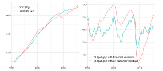
The influence of the import prices and oil prices on inflation in Eq. (9) is assumed to be measured by the average impact over two lagged quarters. In Eq. (11) $u_{t}^{*}$ is assumed to be a constant (exogenous). In the IS curve, the financial variables are assumed to be exogenous and the influence of world demand is captured by the average of the impacts of current and previous quarters $\left(D_{c}^{p_{c}}(L)=0.5 a_{31}\left(L+L^{2}\right.\right.$, $\left.D_{s}^{p_{x}}(L)=0.5 a_{32}\left(L+L^{2}\right), D_{w}^{p_{w}}(L)=0.5(1+L)\right)$. Moreover, we do not consider the influence of the interest rate. Finally potential growth rate is assumed to be a constant (exogenous)
Denoting $\Theta$ the set of parameter to estimate, we, therefore, search for $\hat{\Theta}, \hat{X}{t}$ that minimizes the following loss function: $$ \sum{t=1}^{T}\left{\frac{1}{\sigma_{\tilde{y}}^{2}}\left(y_{t}-y_{t}^{*}\right)^{2}+\frac{1}{\sigma_{y *}^{2}}\left(\epsilon_{t}^{y *}\right)^{2}+\frac{1}{\sigma_{\pi}^{2}}\left(\epsilon_{t}^{\pi}\right)^{2}+\frac{1}{\sigma_{\tilde{u}}^{2}}\left(\epsilon^{\tilde{u}}\right)^{2}\right}
$$
The estimates depends upon the values of the following weights (scaling factors): $\lambda_{1}=\frac{\sigma_{y}^{2}}{\sigma_{y y}^{2}}, \lambda_{2}=\frac{\sigma_{i}^{2}}{\sigma_{\pi}^{2}}, \lambda_{3}=\frac{\sigma_{y}^{2}}{\sigma_{v}^{2}}$. As has been evidenced in the literature, there is no clear guidance about the choice of particular values for these scaling factors. Even the conventional value of 1600 usually chosen for $\lambda_{1}$ would not be appropriate here as the cyclical properties of the output-gap depend upon all the scaling factors. We leave those scaling be estimated by the data. This first-step estimation, with constant $g$ aims at generating some first guess values for the output-gap and the coefficients of the Phillips, IS and Okun equations.
商科代写|计量经济学代写Econometrics代考|The Theoretical Concept of Rational Bubbles
The main objective of this study is to review statistical methods, but it is still important to understand the underlying economic theory of financial bubbles in order to specify a composition of statistical models. As discussed, recent research casts doubt on the rationality of investors, but many economic analyses maintain this assumption and it is often explained using the present value model (PVM). The rationality assumption prevails in academic research largely for convenience; it is easier to model rational behaviors than irrational ones. Survey data on investors’ expectations are the best source of information about investors’ expectations, but in the absence of survey data for a comprehensive number of countries and infrequent dissemination of survey data, we also maintain the rationality assumption.
According to the PVM, rational bubbles are defined as sizable and persistent deviations from economic fundamentals and follow a non-stationary process in a statistical sense. Based on the definition of asset returns or returns on real estate $\left(r_{t+1}=\left(P_{t+1}+D_{t+1}\right) / P_{t}-1\right)$, the PVM suggests that the contemporaneous prices $\left(P_{t}\right)$ will be determined by the expected value of future economic fundamentals $(D)$ and prices:
$$
P_{t}=E_{t}\left[\frac{P_{t+1}+D_{t+1}}{1+r_{t+1}}\right]
$$
where $t$ denotes time $(t=1, \ldots, T)$ and $E$ is an expectation operator. $D$ is an economic fundamental, such as dividend payments in equity analyses or rental costs in housing analyses. Solving Eq. (1) forwardly and using the law of iterated expectations, we can obtain Eq. (2):
$$
P_{t}=E_{t}\left[\sum_{h=0}^{\infty}\left(\prod_{k=0}^{h}\left(\frac{1}{1+r_{t+k}}\right)\right) D_{t+h}+\lim {h \rightarrow \infty} \prod{k=0}^{h}\left(\frac{1}{1+r_{t+k}}\right) P_{t+h}\right]
$$ When $P$ and $D$ are cointegrated, and when the transversality condition holds (i.e., $\left.E_{t}\left[\lim {h \rightarrow \infty} \prod{k=0}^{h}\left(\frac{1}{1+r_{i+k}}\right) P_{t+h}\right] \rightarrow 0\right)$, then the result shows no evidence of bubbles. Therefore, in this case, asset prices tend to move along with the economic fundamentals. On the other hand, when these conditions do not hold, then the results indicate evidence of bubbles. For this reason, prior studies frequently investigated rational bubbles using integration methods.
商科代写|计量经济学代写Econometrics代考|Econometric Methods
Econometricians proposed many statistical methods, with statistical hypotheses that seem designed to be suitable from their perspectives. Consequently, some approaches were developed to look for tranquil periods, while others investigate financial bubbles. Unlike previous studies, we make a clear distinction between statistical approaches to determine tranquil and bubble periods. This distinction is important since differences in the statistical hypotheses can explain the different results from these two approaches. In this section, we will clarify these two approaches using popular statistical specifications in studies of bubbles.
To investigate the theoretical model and predictions in Eq. (2) quantitatively, previous studies often focused on a single market utilizing time series methods. These statistical methods are one-tailed tests, but can be broadly categorized into left- and right-tailed approaches according to their alternative hypotheses. The lefttailed test is classical and is designed to look for cointegration between prices and economic fundamentals, and thus revealing tranquil periods. As an extension, we also propose a nonlinear approach that can be classified into a group of left-tailed tests. On the other hand, the right-tailed test, which has become popular, is an approach to identify explosive bubbles.
计量经济学代考
商科代写|计量经济学代写Econometrics代考|Estimation Method
由于我们有一些未观察到的变量,因此起点是使用状态空间表示来编写模型。然后使用卡尔曼滤波器方法估计参数和未知变量。模型的状态空间表示如下:
X吨=一个X吨−1+从吨+F吨在吨: 状态方程 是吨=μ吨+C吨′X吨+在吨: 测量方程
X吨是向量ķ1状态变量(未观察到),是吨是向量ķ2观察到的变量,A 是ķ1×ķ1矩阵,从我是一个ķ1×1确定性术语的向量,在吨是一个r1×1残差向量,F吨是一个ķ1×r1矩阵,μ吨是一个产品ķ2×n和Xpl由 nexpl 解释变量向量组成的系数矩阵。C吨是一个维度矩阵ķ2×ķ1和在吨是一个向量r2剩余条款。
为了估计模型,我们采用基于五个步骤的顺序方法。
第 1 步:我们用三个状态变量估计模型:是吨,是吨−1,是吨−2∗和三个观察到的变量是吨,圆周率吨,在~吨.
方程中进口价格和石油价格对通货膨胀的影响。(9) 假设通过两个滞后季度的平均影响来衡量。在等式。(11)在吨∗假定为常数(外生的)。在 IS 曲线中,假设金融变量是外生的,世界需求的影响由当前和前几个季度的平均影响来捕捉(DCpC(大号)=0.5一个31(大号+大号2, DspX(大号)=0.5一个32(大号+大号2),D在p在(大号)=0.5(1+大号)). 此外,我们不考虑利率的影响。最后假设潜在增长率是一个常数(外生的)
表示θ要估计的参数集,因此,我们搜索θ^,X^吨最小化以下损失函数:
\sum{t=1}^{T}\left{\frac{1}{\sigma_{\tilde{y}}^{2}}\left(y_{t}-y_{t}^{*} \right)^{2}+\frac{1}{\sigma_{y *}^{2}}\left(\epsilon_{t}^{y *}\right)^{2}+\frac{1 }{\sigma_{\pi}^{2}}\left(\epsilon_{t}^{\pi}\right)^{2}+\frac{1}{\sigma_{\tilde{u}}^ {2}}\left(\epsilon^{\tilde{u}}\right)^{2}\right}\sum{t=1}^{T}\left{\frac{1}{\sigma_{\tilde{y}}^{2}}\left(y_{t}-y_{t}^{*} \right)^{2}+\frac{1}{\sigma_{y *}^{2}}\left(\epsilon_{t}^{y *}\right)^{2}+\frac{1 }{\sigma_{\pi}^{2}}\left(\epsilon_{t}^{\pi}\right)^{2}+\frac{1}{\sigma_{\tilde{u}}^ {2}}\left(\epsilon^{\tilde{u}}\right)^{2}\right}
估计值取决于以下权重(比例因子)的值:λ1=σ是2σ是是2,λ2=σ一世2σ圆周率2,λ3=σ是2σ在2. 正如文献中所证明的,对于这些比例因子的特定值的选择没有明确的指导。即使是通常选择的 1600 的常规值λ1在这里不合适,因为输出差距的周期性属性取决于所有比例因子。我们让这些缩放由数据来估计。第一步估计,常数G旨在为输出间隙和 Phillips、IS 和 Okun 方程的系数生成一些初步猜测值。
商科代写|计量经济学代写Econometrics代考|The Theoretical Concept of Rational Bubbles
本研究的主要目的是回顾统计方法,但理解金融泡沫的基本经济理论以指定统计模型的组成仍然很重要。正如所讨论的,最近的研究对投资者的理性提出了质疑,但许多经济分析都维持了这一假设,并且通常使用现值模型 (PVM) 来解释。理性假设在学术研究中盛行,主要是为了方便。对理性行为进行建模比对非理性行为进行建模更容易。投资者预期的调查数据是投资者预期信息的最佳来源,但在缺乏全面的国家调查数据和不经常发布的调查数据的情况下,我们也维持理性假设。
根据 PVM,理性泡沫被定义为与经济基本面相当大且持续存在的偏差,并且在统计意义上遵循非平稳过程。基于资产收益或房地产收益的定义(r吨+1=(磷吨+1+D吨+1)/磷吨−1), PVM 表明同期价格(磷吨)将由未来经济基本面的预期值决定(D)和价格:
磷吨=和吨[磷吨+1+D吨+11+r吨+1]
在哪里吨表示时间(吨=1,…,吨)和和是期望算子。D是经济基础,例如股权分析中的股息支付或住房分析中的租金成本。求解方程。(1) 向前并使用迭代期望定律,我们可以得到方程。(2):
磷吨=和吨[∑H=0∞(∏ķ=0H(11+r吨+ķ))D吨+H+林H→∞∏ķ=0H(11+r吨+ķ)磷吨+H]什么时候磷和D是协整的,并且当横向条件成立时(即,和吨[林H→∞∏ķ=0H(11+r一世+ķ)磷吨+H]→0),则结果显示没有气泡的迹象。因此,在这种情况下,资产价格往往会随着经济基本面而波动。另一方面,当这些条件不成立时,结果表明存在泡沫。出于这个原因,先前的研究经常使用积分方法研究理性气泡。
商科代写|计量经济学代写Econometrics代考|Econometric Methods
计量经济学家提出了许多统计方法,其统计假设似乎从他们的角度来看是合适的。因此,开发了一些方法来寻找平静时期,而另一些方法则研究金融泡沫。与以前的研究不同,我们明确区分了确定平静期和泡沫期的统计方法。这种区别很重要,因为统计假设的差异可以解释这两种方法的不同结果。在本节中,我们将使用气泡研究中流行的统计规范来阐明这两种方法。
研究方程式中的理论模型和预测。(2) 在数量上,以往的研究往往侧重于利用时间序列方法的单一市场。这些统计方法是单尾检验,但可以根据其替代假设大致分为左尾方法和右尾方法。左尾检验是经典的,旨在寻找价格和经济基本面之间的协整,从而揭示平静时期。作为扩展,我们还提出了一种非线性方法,可以分为一组左尾测试。另一方面,流行的右尾测试是一种识别爆炸气泡的方法。

统计代写请认准statistics-lab™. statistics-lab™为您的留学生涯保驾护航。
金融工程代写
金融工程是使用数学技术来解决金融问题。金融工程使用计算机科学、统计学、经济学和应用数学领域的工具和知识来解决当前的金融问题,以及设计新的和创新的金融产品。
非参数统计代写
非参数统计指的是一种统计方法,其中不假设数据来自于由少数参数决定的规定模型;这种模型的例子包括正态分布模型和线性回归模型。
广义线性模型代考
广义线性模型(GLM)归属统计学领域,是一种应用灵活的线性回归模型。该模型允许因变量的偏差分布有除了正态分布之外的其它分布。
术语 广义线性模型(GLM)通常是指给定连续和/或分类预测因素的连续响应变量的常规线性回归模型。它包括多元线性回归,以及方差分析和方差分析(仅含固定效应)。
有限元方法代写
有限元方法(FEM)是一种流行的方法,用于数值解决工程和数学建模中出现的微分方程。典型的问题领域包括结构分析、传热、流体流动、质量运输和电磁势等传统领域。
有限元是一种通用的数值方法,用于解决两个或三个空间变量的偏微分方程(即一些边界值问题)。为了解决一个问题,有限元将一个大系统细分为更小、更简单的部分,称为有限元。这是通过在空间维度上的特定空间离散化来实现的,它是通过构建对象的网格来实现的:用于求解的数值域,它有有限数量的点。边界值问题的有限元方法表述最终导致一个代数方程组。该方法在域上对未知函数进行逼近。[1] 然后将模拟这些有限元的简单方程组合成一个更大的方程系统,以模拟整个问题。然后,有限元通过变化微积分使相关的误差函数最小化来逼近一个解决方案。
tatistics-lab作为专业的留学生服务机构,多年来已为美国、英国、加拿大、澳洲等留学热门地的学生提供专业的学术服务,包括但不限于Essay代写,Assignment代写,Dissertation代写,Report代写,小组作业代写,Proposal代写,Paper代写,Presentation代写,计算机作业代写,论文修改和润色,网课代做,exam代考等等。写作范围涵盖高中,本科,研究生等海外留学全阶段,辐射金融,经济学,会计学,审计学,管理学等全球99%专业科目。写作团队既有专业英语母语作者,也有海外名校硕博留学生,每位写作老师都拥有过硬的语言能力,专业的学科背景和学术写作经验。我们承诺100%原创,100%专业,100%准时,100%满意。
随机分析代写
随机微积分是数学的一个分支,对随机过程进行操作。它允许为随机过程的积分定义一个关于随机过程的一致的积分理论。这个领域是由日本数学家伊藤清在第二次世界大战期间创建并开始的。
时间序列分析代写
随机过程,是依赖于参数的一组随机变量的全体,参数通常是时间。 随机变量是随机现象的数量表现,其时间序列是一组按照时间发生先后顺序进行排列的数据点序列。通常一组时间序列的时间间隔为一恒定值(如1秒,5分钟,12小时,7天,1年),因此时间序列可以作为离散时间数据进行分析处理。研究时间序列数据的意义在于现实中,往往需要研究某个事物其随时间发展变化的规律。这就需要通过研究该事物过去发展的历史记录,以得到其自身发展的规律。
回归分析代写
多元回归分析渐进(Multiple Regression Analysis Asymptotics)属于计量经济学领域,主要是一种数学上的统计分析方法,可以分析复杂情况下各影响因素的数学关系,在自然科学、社会和经济学等多个领域内应用广泛。
MATLAB代写
MATLAB 是一种用于技术计算的高性能语言。它将计算、可视化和编程集成在一个易于使用的环境中,其中问题和解决方案以熟悉的数学符号表示。典型用途包括:数学和计算算法开发建模、仿真和原型制作数据分析、探索和可视化科学和工程图形应用程序开发,包括图形用户界面构建MATLAB 是一个交互式系统,其基本数据元素是一个不需要维度的数组。这使您可以解决许多技术计算问题,尤其是那些具有矩阵和向量公式的问题,而只需用 C 或 Fortran 等标量非交互式语言编写程序所需的时间的一小部分。MATLAB 名称代表矩阵实验室。MATLAB 最初的编写目的是提供对由 LINPACK 和 EISPACK 项目开发的矩阵软件的轻松访问,这两个项目共同代表了矩阵计算软件的最新技术。MATLAB 经过多年的发展,得到了许多用户的投入。在大学环境中,它是数学、工程和科学入门和高级课程的标准教学工具。在工业领域,MATLAB 是高效研究、开发和分析的首选工具。MATLAB 具有一系列称为工具箱的特定于应用程序的解决方案。对于大多数 MATLAB 用户来说非常重要,工具箱允许您学习和应用专业技术。工具箱是 MATLAB 函数(M 文件)的综合集合,可扩展 MATLAB 环境以解决特定类别的问题。可用工具箱的领域包括信号处理、控制系统、神经网络、模糊逻辑、小波、仿真等。