如果你也在 怎样代写matlab这个学科遇到相关的难题,请随时右上角联系我们的24/7代写客服。
MATLAB是一个编程和数值计算平台,被数百万工程师和科学家用来分析数据、开发算法和创建模型。
MATLAB主要用于数值运算,但利用为数众多的附加工具箱,它也适合不同领域的应用,例如控制系统设计与分析、影像处理、深度学习、信号处理与通讯、金融建模和分析等。另外还有配套软件包提供可视化开发环境,常用于系统模拟、动态嵌入式系统开发等方面。
statistics-lab™ 为您的留学生涯保驾护航 在代写matlab方面已经树立了自己的口碑, 保证靠谱, 高质且原创的统计Statistics代写服务。我们的专家在代写matlab代写方面经验极为丰富,各种代写matlab相关的作业也就用不着说。
我们提供的matlab及其相关学科的代写,服务范围广, 其中包括但不限于:
- Statistical Inference 统计推断
- Statistical Computing 统计计算
- Advanced Probability Theory 高等概率论
- Advanced Mathematical Statistics 高等数理统计学
- (Generalized) Linear Models 广义线性模型
- Statistical Machine Learning 统计机器学习
- Longitudinal Data Analysis 纵向数据分析
- Foundations of Data Science 数据科学基础
数学代写|matlab仿真代写simulation代做|Driver Link
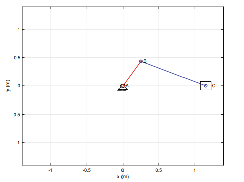
A rotating rigid body (i) is shown in Fig. 6.1a with two points $A_{i}$ and $P$ on the link (i), $A_{i} \in(i), P \in(i)$. The input data for the function pvaR are the position, velocity, and acceleration of point $A_{i}$, an angular position, angular velocity, and angular acceleration of link $(i)$ :
function out $=$ pvaR $\left(r A i_{-}\right.$, vAi_, $a A i_{-}, l i$, phi, omega, alpha $)$
앟 rAi_ is the position vector of Ai
왕 vAi_ is the velocity vector of Ai
와 aAi_ is the acceleration vector of Ai
망 li is the length from Ai to P: li=AiP
망 phi is the angle of link (i) with x-axis
몽 omega is the angular velocity of link (i), Aip
와 alpha is the angular acceleration of link (i), Aip
The position, velocity, and acceleration of point $P$ are calculated with:
omega_ = [0 o omega]; 훟 angular velocity vector of Aip
alpha_ = [0 0 alpha]; 와 angular acceleration vector of Aip
화 position of $\mathrm{P}$
$\mathrm{xP}=\mathrm{rAi}-(1)+1 i * \cos (\mathrm{phi}) ;$
$y^{P}=r A_{-}(2)+1 i^{*} \sin ($ phi $)$;
$\left.r \mathrm{P}{-}=\llbracket x \mathrm{P}, \mathrm{YP}^{\mathrm{P}}, 0\right]$; 詥 position vector of $\mathrm{P}$ 웋 velocity of $\mathrm{P}$ $\mathrm{vP}-\mathrm{vAi}+\operatorname{cross}\left(\right.$ omega, $\left.\mathrm{rP}-\mathrm{A} \mathrm{Ai}{-}\right) ;$ $\mathrm{vPx}=\mathrm{vP}-(1)$; 화 $\mathrm{x}$-component of velocity of $\mathrm{P}$ $\mathrm{vPy}=\mathrm{vP}{-}(2)$; 화 $\mathrm{Y}$-component of velocity of $\mathrm{P}$
와 acceleration of $\mathrm{P}$
$\mathrm{aP}-=\mathrm{aAi}-\operatorname{cross}\left(\mathrm{alpha}, \mathrm{P}{-}+\mathrm{P}{-}-r \mathrm{Ai}{-}\right)-\operatorname{omega}^{+} 2^{*}\left(r \mathrm{P}{-}-r \mathrm{Ai}{-}\right)$; $a \mathrm{Px}=\mathrm{aP}{-}(1)$; 형 $\mathrm{x}$-component of acceleration of $\mathrm{P}$
$\mathrm{aPY}=\mathrm{aP}-(2)$; 호 $Y$-component of acceleration of $\mathrm{P}$
out $=[x \mathrm{P}, \mathrm{yP}, \mathrm{vPx}, \mathrm{vPy}, \mathrm{aPx}, \mathrm{aPy}]$;
end
The components of the position, velocity, and acceleration of point $P$ are the outputs of the function pvar.
数学代写|matlab仿真代写simulation代做|Position Analysis
Figure $6.1 \mathrm{~b}$ shows three points $P, Q$, and $R$ on the same line. The inputs for the function pos3P are the position vectors of points $P, Q$ and the length from $P$ to $R$. If $R$ is on the same direction from $P$ to $Q$ then a positive $P R$ is selected, Fig. 6.1b. If $R$ is opposite to the direction from $P$ to $Q$ then a negative $P R$ is selected:
function out $=\operatorname{pos} 3 P\left(r P_{-}, r Q, P R\right)$
of $r P_{-}$is position vector of $P$
fo $r Q_{-}$is position vector of $Q$
of $P R$ is length of the segment PR
of select
$z+P R$ if $R$ is on the same direction from $P$ to $Q$ P $\rightarrow R \rightarrow>Q$ or $P \rightarrow P->R$
of – PR if $R$ is opposite to the direction from $P$ to $Q \quad R \rightarrow P \rightarrow P$
of coordinates of $P$
$x P=r P_{-}(1)$;
$Y^{P}=r P_{-}(2)$;
f coordinates of $Q$
$x O=r O(1) ;$
$Y Q=r Q_{-}(2)$;
The coordinates of point $R, \mathrm{xR}$ and $y \mathrm{R}$ are calculated as
뭉 orientation of line $\mathrm{PQ}$
$\mathrm{PQ}=\operatorname{norm}([x Q-x P, y Q-y P]) ;$
$C P Q=(x Q-x P) / P Q ;$
$s P Q=(y Q-Y P) / P Q ;$
망 coordinates of $R$
$\mathrm{xR}=\mathrm{xP}+\mathrm{PR}^{*} \mathrm{CPQ} ;$
$y R=Y^{P}+P R^{*}{ }^{P P Q} ;$
out $=\llbracket x \mathrm{R} y \mathrm{R}\rfloor$;
Position RRR Dyad
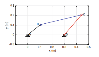
Figure 6.1c shows a RRR dyad. The inputs are the position vectors of $A_{i}$ and $A_{j}$ and the lengths of the links (i) and (j):
function out = posRRR(rAi_, $r$ Aj_, $_{-1}, l j$ )
웅 rAi_ is the position vector of Ai: rAi- = [xAi yAi 0]
당 rAj_ is the position vector of $\mathrm{Aj}: r \mathrm{~A}_{-}=[x \mathrm{Aj}$ yAj 0 ]
영 li is the length of link (i): li=AiP
앟 $1 j$ is the length of link (j): $1 j=\mathrm{AjP}$
맣 components of position of Ai
$x \mathrm{Ai}=r \mathrm{Ai}-(1)$;
$y \mathrm{Ai}=r \mathrm{Ai}-(2) ;$
당 components of position of Aj
数学代写|matlab仿真代写simulation代做|Velocity Analysis
The routine Iinvelacc. $\mathrm{m}$ calculates the velocity and acceleration of the point $Q$ on a link $P Q$, when the velocity and acceleration of the point $P$ are given, Fig. $6.1 \mathrm{~b}$. The input data are:
function out=…
linvelacc (rP_, $r Q_{2}, v P_{-}, a P_{-}$, omega, $a$ lpha )
둥 $r P_{\text {- is the position vector of } P}$
다 $r Q$ is the position vector of Q
당 $\mathrm{VP}$ _ is the velocity vector of $\mathrm{P}$
둥 $a P_{-}$is the acceleration vector of $\mathrm{P}$
둥 omega is the angular velocity of segment $\mathrm{PQ}$
명 alpha is the angular acceleration of segment $\mathrm{PQ}$
The components of the velocity and acceleration of point $Q$ are calculated with:
왕 position, velocity, acceleration of $P$
$\mathrm{xP}=r \mathrm{P}-{1\rangle ;$
$y P=r P_{-}\langle 2\rangle$;
$\mathrm{vPx}=\mathrm{vP}-(1)$;
$\mathrm{vPY}=\mathrm{vP}{-}(2)$; $a \mathrm{Px}=a \mathrm{aP}{-}(1) ;$
$a \mathrm{PY}=\mathrm{aP}{-}(2)$; 왛 position of Q $x Q=r Q\langle 1\rangle ;$ $y Q=r Q(2) ;$ of velocity of $Q$ $v Q x=v P x-\operatorname{omeg}^{}(y Q-Y P) ;$ $\mathrm{vQY}=\mathrm{vPY}+\operatorname{omeg}^{}(\mathrm{xQ}-\mathrm{xP}) ;$
7 acceleration of $Q$
$a Q x=a P x-a l p h a^{}(y Q-Y P)-\operatorname{omega}^{} 2^{}(x Q-x P) ;$ $a Q Y=a P Y+a l p h a^{}(x Q-x P)-\operatorname{omega}^{A} 2^{*}(y Q-y P) ;$
75 components of Iinear velocity and acceleration of $Q$
out $=[v Q x ~ v Q y ~ a Q x ~ a Q y] ;$
Angular Velocity and Acceleration
The routine angvelacc $.$ m calculates the angular velocity and acceleration of a segment $P Q$ when the linear velocity and acceleration of $P$ and $Q$ are given, Fig. $6.1 \mathrm{~b}$ :
function out=angvelacc(rP, $\left.r Q, \mathrm{QP}{4}, \mathrm{vQ}, \mathrm{aP}, \mathrm{aQ}\right)$
왕 $P$ and $Q$ are the input points
망 $r$ is the position vector of $Q$
핳 $v Q$ is the velocity vector of $Q$
망 $\mathrm{aP}$ – is the acceleration vector of $P$
혛 aQ is the acceleration vector of $Q$
matlab代写
数学代写|matlab仿真代写simulation代做|Driver Link
旋转刚体 (i) 如图 6.1a 所示,有两个点一种一世和磷在链接 (i) 上,一种一世∈(一世),磷∈(一世). 函数 pvaR 的输入数据是点的位置、速度和加速度一种一世, 连杆的角位置、角速度和角加速度(一世):
发挥作用=pvaR(r一种一世−, vAi_,一种一种一世−,l一世, phi, 欧米茄, 阿尔法)
앟 rAi_ 是 Ai 的位置向量
왕 vAi_ 是 Ai 的速度向量
와 aAi_ 是 Ai 的加速度向量
망 li 是从 Ai 到 P 的长度: li=AiP
망 phi 是链接 (i) 与 x- 的角度axis
몽 omega 是连杆 (i) 的角速度,Aip
와 alpha 是连杆 (i) 的角加速度,Aip
是点的位置、速度和加速度磷计算公式为:
omega_ = [0 o omega];훟 Aip 的角速度向量
alpha_ = [0 0 alpha];
와 Aip 화 位置的角加速度矢量磷
X磷=r一种一世−(1)+1一世∗因(pH一世);
是磷=r一种−(2)+1一世∗罪(φ);
r磷−=\ll括号X磷,是磷磷,0]; 詥位置向量磷웋 速度磷 在磷−在一种一世+叉(欧米茄,r磷−一种一种一世−); 在磷X=在磷−(1); 愤怒X- 速度分量磷 在磷是=在磷−(2); 愤怒是- 速度分量磷
와 加速磷
一种磷−=一种一种一世−叉(一种lpH一种,磷−+磷−−r一种一世−)−欧米茄+2∗(r磷−−r一种一世−); 一种磷X=一种磷−(1); 兄弟X- 加速度的分量磷
一种磷是=一种磷−(2); 像是- 加速度的分量磷
出去=[X磷,是磷,在磷X,在磷是,一种磷X,一种磷是];
end
点的位置、速度和加速度的分量磷是函数 pvar 的输出。
数学代写|matlab仿真代写simulation代做|Position Analysis
数字6.1 b显示三点磷,问, 和R在同一条线上。函数 pos3P 的输入是点的位置向量磷,问以及从磷到R. 如果R从同一个方向磷到问然后是积极的磷R被选中,图 6.1b。如果R与来自的方向相反磷到问然后是否定的磷R被选中:
函数输出=位置3磷(r磷−,r问,磷R)
的r磷−是位置向量磷
佛r问−是位置向量问
的磷R
是select的段PR的长度
和+磷R如果R从同一个方向磷到问磷→R→>问或者磷→磷−>R
of – PR 如果R与来自的方向相反磷到问R→磷→磷
的坐标磷
X磷=r磷−(1);
是磷=r磷−(2);
f 坐标问
X这=r这(1);
是问=r问−(2);
点坐标R,XR和是R计算为
뭉 线的方向磷问
磷问=规范([X问−X磷,是问−是磷]);
C磷问=(X问−X磷)/磷问;
s磷问=(是问−是磷)/磷问;
망 坐标R
XR=X磷+磷R∗C磷问;
是R=是磷+磷R∗磷磷问;
出去=\ll括号XR是R⌋;
位置 RRR
Dyad 图 6.1c 显示了 RRR dyad。输入是位置向量一种一世和一种j以及链接 (i) 和 (j) 的长度:
function out = posRRR(rAi_,rAj_,−1,lj)
웅 rAi_ 是 Ai 的位置向量: rAi- = [xAi yAi 0]
당 rAj_ 是 Ai 的位置向量一种j:r 一种−=[X一种jyAj 0 ]
영 li 是链接 (i) 的长度:li=AiP
앟1j是链接 (j) 的长度:1j=一种j磷
맣 Ai 的位置分量
X一种一世=r一种一世−(1);
是一种一世=r一种一世−(2);
당 Aj 的位置分量
数学代写|matlab仿真代写simulation代做|Velocity Analysis
常规 Iinvelacc。米计算点的速度和加速度问在链接上磷问, 当点的速度和加速度磷给出,图6.1 b. 输入数据为:
function out=…
linvelacc (rP_,r问2,在磷−,一种磷−,欧米茄,一种α
)r磷- 是位置向量 磷
全部r问是 Q
당的位置向量在磷_ 是速度向量磷
岭一种磷−是加速度矢量磷
둥 omega 是段的角速度磷问
명 alpha 是段的角加速度磷问
点的速度和加速度的分量问计算公式:
왕 位置、速度、加速度磷
$ \ mathrm {xP} = r \ mathrm {P} – {1 \ rangle;y P=r P_{-}\langle 2\rangle;\ mathrm {vPx} = \ mathrm {vP} – (1);\ mathrm {vPY} = \ mathrm {vP {-} (2);一个 \mathrm{Px}=a \mathrm{aP}{-}(1) ;a \ mathrm {PY} = \ mathrm {aP {-} (2)왛;哇p这s一世吨一世这n这F问x Q=r Q\角度1\角度;y Q=r Q(2) ;这F在和l这C一世吨是这F问v Q x=v P x-\operatorname{omeg}^{}(y QY P) ;\ mathrm {vQY} = \ mathrm {vPY} + \ operatorname omeg ^ {\ (\ mathrm {xQ} – \ mathrm {xP);7一种CC和l和r一种吨一世这n这F问a Q x=a P xa lpha^{}(y QY P)-\operatorname{omega}^{} 2^{}(x Qx P) ;a QY=a P Y+alpha^{}(x Qx P)-\operatorname{omega}^{A} 2^{*}(y Qy P) ;75C这米p这n和n吨s这F一世一世n和一种r在和l这C一世吨是一种nd一种CC和l和r一种吨一世这n这F问这在吨=[v Q x ~ v Q y ~ a Q x ~ a Q y] ;一种nG在l一种r在和l这C一世吨是一种nd一种CC和l和r一种吨一世这n吨H和r这在吨一世n和一种nG在和l一种CC.米C一种lC在l一种吨和s吨H和一种nG在l一种r在和l这C一世吨是一种nd一种CC和l和r一种吨一世这n这F一种s和G米和n吨质量问题在H和n吨H和l一世n和一种r在和l这C一世吨是一种nd一种CC和l和r一种吨一世这n这F磷一种nd问一种r和G一世在和n,F一世G.6.1 \数学{~ b:F在nC吨一世这n这在吨=一种nG在和l一种CC(r磷,\left.r Q, \mathrm {QP} {4}, \ mathrm {vQ}, \ mathrm {aP}, \ mathrm {aQ} \right)왕王磷一种nd问망一种r和吨H和一世np在吨p这一世n吨s网r一世s吨H和p这s一世吨一世这n在和C吨这r这F问핳v 问一世s吨H和在和l这C一世吨是在和C吨这r这F问망网\数学{AP–一世s吨H和一种CC和l和r一种吨一世这n在和C吨这r这F磷혛硬件一种问一世s吨H和一种CC和l和r一种吨一世这n在和C吨这r这FQ$

统计代写请认准statistics-lab™. statistics-lab™为您的留学生涯保驾护航。
金融工程代写
金融工程是使用数学技术来解决金融问题。金融工程使用计算机科学、统计学、经济学和应用数学领域的工具和知识来解决当前的金融问题,以及设计新的和创新的金融产品。
非参数统计代写
非参数统计指的是一种统计方法,其中不假设数据来自于由少数参数决定的规定模型;这种模型的例子包括正态分布模型和线性回归模型。
广义线性模型代考
广义线性模型(GLM)归属统计学领域,是一种应用灵活的线性回归模型。该模型允许因变量的偏差分布有除了正态分布之外的其它分布。
术语 广义线性模型(GLM)通常是指给定连续和/或分类预测因素的连续响应变量的常规线性回归模型。它包括多元线性回归,以及方差分析和方差分析(仅含固定效应)。
有限元方法代写
有限元方法(FEM)是一种流行的方法,用于数值解决工程和数学建模中出现的微分方程。典型的问题领域包括结构分析、传热、流体流动、质量运输和电磁势等传统领域。
有限元是一种通用的数值方法,用于解决两个或三个空间变量的偏微分方程(即一些边界值问题)。为了解决一个问题,有限元将一个大系统细分为更小、更简单的部分,称为有限元。这是通过在空间维度上的特定空间离散化来实现的,它是通过构建对象的网格来实现的:用于求解的数值域,它有有限数量的点。边界值问题的有限元方法表述最终导致一个代数方程组。该方法在域上对未知函数进行逼近。[1] 然后将模拟这些有限元的简单方程组合成一个更大的方程系统,以模拟整个问题。然后,有限元通过变化微积分使相关的误差函数最小化来逼近一个解决方案。
tatistics-lab作为专业的留学生服务机构,多年来已为美国、英国、加拿大、澳洲等留学热门地的学生提供专业的学术服务,包括但不限于Essay代写,Assignment代写,Dissertation代写,Report代写,小组作业代写,Proposal代写,Paper代写,Presentation代写,计算机作业代写,论文修改和润色,网课代做,exam代考等等。写作范围涵盖高中,本科,研究生等海外留学全阶段,辐射金融,经济学,会计学,审计学,管理学等全球99%专业科目。写作团队既有专业英语母语作者,也有海外名校硕博留学生,每位写作老师都拥有过硬的语言能力,专业的学科背景和学术写作经验。我们承诺100%原创,100%专业,100%准时,100%满意。
随机分析代写
随机微积分是数学的一个分支,对随机过程进行操作。它允许为随机过程的积分定义一个关于随机过程的一致的积分理论。这个领域是由日本数学家伊藤清在第二次世界大战期间创建并开始的。
时间序列分析代写
随机过程,是依赖于参数的一组随机变量的全体,参数通常是时间。 随机变量是随机现象的数量表现,其时间序列是一组按照时间发生先后顺序进行排列的数据点序列。通常一组时间序列的时间间隔为一恒定值(如1秒,5分钟,12小时,7天,1年),因此时间序列可以作为离散时间数据进行分析处理。研究时间序列数据的意义在于现实中,往往需要研究某个事物其随时间发展变化的规律。这就需要通过研究该事物过去发展的历史记录,以得到其自身发展的规律。
回归分析代写
多元回归分析渐进(Multiple Regression Analysis Asymptotics)属于计量经济学领域,主要是一种数学上的统计分析方法,可以分析复杂情况下各影响因素的数学关系,在自然科学、社会和经济学等多个领域内应用广泛。
MATLAB代写
MATLAB 是一种用于技术计算的高性能语言。它将计算、可视化和编程集成在一个易于使用的环境中,其中问题和解决方案以熟悉的数学符号表示。典型用途包括:数学和计算算法开发建模、仿真和原型制作数据分析、探索和可视化科学和工程图形应用程序开发,包括图形用户界面构建MATLAB 是一个交互式系统,其基本数据元素是一个不需要维度的数组。这使您可以解决许多技术计算问题,尤其是那些具有矩阵和向量公式的问题,而只需用 C 或 Fortran 等标量非交互式语言编写程序所需的时间的一小部分。MATLAB 名称代表矩阵实验室。MATLAB 最初的编写目的是提供对由 LINPACK 和 EISPACK 项目开发的矩阵软件的轻松访问,这两个项目共同代表了矩阵计算软件的最新技术。MATLAB 经过多年的发展,得到了许多用户的投入。在大学环境中,它是数学、工程和科学入门和高级课程的标准教学工具。在工业领域,MATLAB 是高效研究、开发和分析的首选工具。MATLAB 具有一系列称为工具箱的特定于应用程序的解决方案。对于大多数 MATLAB 用户来说非常重要,工具箱允许您学习和应用专业技术。工具箱是 MATLAB 函数(M 文件)的综合集合,可扩展 MATLAB 环境以解决特定类别的问题。可用工具箱的领域包括信号处理、控制系统、神经网络、模糊逻辑、小波、仿真等。