如果你也在 怎样代写matlab这个学科遇到相关的难题,请随时右上角联系我们的24/7代写客服。
MATLAB是一个编程和数值计算平台,被数百万工程师和科学家用来分析数据、开发算法和创建模型。
MATLAB主要用于数值运算,但利用为数众多的附加工具箱,它也适合不同领域的应用,例如控制系统设计与分析、影像处理、深度学习、信号处理与通讯、金融建模和分析等。另外还有配套软件包提供可视化开发环境,常用于系统模拟、动态嵌入式系统开发等方面。
statistics-lab™ 为您的留学生涯保驾护航 在代写matlab方面已经树立了自己的口碑, 保证靠谱, 高质且原创的统计Statistics代写服务。我们的专家在代写matlab代写方面经验极为丰富,各种代写matlab相关的作业也就用不着说。
我们提供的matlab及其相关学科的代写,服务范围广, 其中包括但不限于:
- Statistical Inference 统计推断
- Statistical Computing 统计计算
- Advanced Probability Theory 高等概率论
- Advanced Mathematical Statistics 高等数理统计学
- (Generalized) Linear Models 广义线性模型
- Statistical Machine Learning 统计机器学习
- Longitudinal Data Analysis 纵向数据分析
- Foundations of Data Science 数据科学基础
数学代写|matlab仿真代写simulation代做|Planar Dynamics Analysis
Consider an arbitrary rigid body in motion with the total mass $m$. The position of the mass center of the rigid body is $\mathbf{r}{C}$ and $\mathbf{a}{C}$ is the acceleration of the mass center $C$. The sum of the external forces, $\mathbf{F}$, acting on the system equals the product of the mass and the acceleration of the mass center
$$
m \mathbf{a}{C}=\mathbf{F} $$ Equation (1.44) is Newton’s second law for a rigid body and is applicable to planar and three-dimensional motions. Resolving the sum of the external forces into Cartesian rectangular components $$ \mathbf{F}=F{x} \mathbf{1}+F_{y} \mathbf{J}+F_{z} \mathbf{k}
$$
and the position vector of the mass center
$$
\mathbf{r}{C}=x{C}(t) \mathbf{1}+y_{C}(t) \mathbf{j}+z_{C}(t) \mathbf{k},
$$
Newton’s second law for the rigid body is
$$
m \ddot{\mathbf{r}}{C}=\mathbf{F} $$ or $$ m \ddot{x}{C}=F_{x}, \quad m \ddot{y}{C}=F{y}, \quad m \ddot{z}{C}=F{z} .
$$
Figure $1.14$ shows a rigid body moving in the $(x, y)$ plane with the origin at $O$. The mass center $C$ of the rigid body is in the plane of the motion. The axis $O z$ is perpendicular to the plane of motion of the rigid body, where $O$ is the origin. The axis $C z$ is perpendicular to the plane of motion through the mass center $C$. The angular velocity vector of the rigid body is $\omega=\omega \mathbf{k}$ and the angular acceleration is $\alpha=\dot{\omega}=\ddot{\theta} \mathbf{k}$, where the angle $\theta$ is the angular position of the rigid body about a fixed axis. The mass moment of inertia of the rigid body about the $z$-axis through $C$ is also the polar mass moment of inertia of the rigid body about $C, I_{C z}=I_{C}$.
The rotational equation (Euler’s equation) of motion for the rigid body is
$$
I_{C} \boldsymbol{\alpha}=\sum \mathbf{M}{C}, $$ where $\mathbf{M}{C}$ is the sum of the moments about $C$ due to external forces and couples.
Consider the case when the rigid body rotates about a fixed point $P$. The mass moment of inertia of the rigid body about the $z$-axis through $P$ is (parallel-axis theorem)
$$
I_{P z}=I_{C z}+m(C P)^{2}
$$
For the rigid body rotation about a fixed point $P$, Euler’s equation is
$$
I_{P z} \boldsymbol{\alpha}=\sum \mathbf{M}{P} $$ where $\mathbf{M}{P}$ is the sum of the moments about the fixed point $P$ due to external forces and couples.
数学代写|matlab仿真代写simulation代做|One Dyad
Abstract The planar motion of a mechanism with three moving links is analyzed. Symbolical and numerical MATLAB are used for the kinematics and dynamics of the system. The classical vectorial equations for velocity and acceleration of the rigid body are used. The joint reaction forces and the moment applied to the driver link are calculated for a given position with Newton-Euler equations for inverse dynamics.
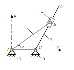
The planar R-RTR mechanism considered is shown in Fig. 2.1. The driver link is the rigid link 1 (the link $A B)$. The dyad RTR $\left(B_{\mathrm{R}}, B_{\mathrm{T}}, C_{\mathrm{R}}\right)$ is composed of the slider 2 and the rocker 3 . The following numerical data are given: $A B=0.10 \mathrm{~m}$, $A C=0.05 \mathrm{~m}$, and $C D=0.15 \mathrm{~m}$. The angle of the driver link 1 with the horizontal axis is $\phi=30^{\circ}$. The constant angular speed of the driver link 1 is $-50 \mathrm{rpm}$.
Given an external moment $\mathbf{M}{c}=-100 \operatorname{sign}\left(\omega{3}\right) \mathbf{k} \mathrm{Nm}$ applied on the link 3 , calculate the motor moment $\mathbf{M}{m}$ required for the dynamic equilibrium of the mechanism. All three links are rectangular prisms with the depth $d=0.001 \mathrm{~m}$ and the mass density $\rho=8000 \mathrm{~kg} / \mathrm{m}^{3}$. The height of the links 1 and 3 is $h=0.01 \mathrm{~m}$. The slider 2 has the height $h{S}=0.02 \mathrm{~m}$, and the width $w_{S}=0.04 \mathrm{~m}$. The center of mass location of the links $i=1,2,3$ are designated by $C_{i}\left(x_{C_{i}}, y_{C_{i}}, 0\right)$. The gravitational acceleration is $g=9.807 \mathrm{~m} / \mathrm{s}^{2}$.
数学代写|matlab仿真代写simulation代做|Position Analysis
A Cartesian reference frame $x y$ is selected. The joint $A$ is in the origin of the reference frame, that is, $A \equiv O$,
$$
x_{A}=0 \text { and } y_{A}=0 .
$$
The coordinates of the joint $C$ are
$$
x_{C}=A C=0.05 \text { and } y_{C}=0 \mathrm{~m} .
$$
Position of joint $B$
The unknowns are the coordinates of the joint $B, x_{B}$ and $y_{B}$. Because the joint $A$ is fixed and the angle $\phi$ is known, the coordinates of the joint $B$ are computed from the following expressions
$$
\begin{aligned}
&x_{B}=A B \cos \phi=0.10 \cos 30^{\circ}=0.087 \mathrm{~m} \
&y_{B}=A B \sin \phi=0.10 \sin 30^{\circ}=0.050 \mathrm{~m}
\end{aligned}
$$
The MATLAB commands for joints $A, C$, and $B$ are:
$A B=0.10 ; \quad$ 읳 $(\mathrm{m})$
$A C=0.05 ; \quad$ 읳 $(\mathrm{m})$
$C D=0.15 ;$ 앟 (m)
phi $=$ pi $/ 6 ;$ 웋 (rad)
$x A=0 ; y A=0$;
$r A_{-}=[x A y A l] ;$
$x C=A C ; y C=0$;
$r C_{-}=[x C y C 0] ;$
$\mathrm{xB}=A \mathrm{~B}^{} \cos ($ phi $)$; $y B=A B^{} \sin ($ phi $)$;
$r B_{-}=[x B y B 0] ;$
Angle $\phi_{2}$
The angle of link 2 (or link 3 ) with the horizontal axis is calculated from the slope of the straight line $B C$ :
$$
\phi_{2}=\phi_{3}=\arctan \frac{y_{B}-y_{C}}{x_{B}-x_{C}}=\arctan \frac{0.050}{0.087-0.050}=0.939 \mathrm{rad}=53.794^{\circ}
$$
matlab代写
数学代写|matlab仿真代写simulation代做|Planar Dynamics Analysis
考虑一个具有总质量的运动中的任意刚体米. 刚体质心的位置为rC和一种C是质心的加速度C. 外力的总和,F, 作用在系统上等于质量和质心加速度的乘积
米一种C=F方程 (1.44) 是刚体的牛顿第二定律,适用于平面和三维运动。将外力的总和分解为笛卡尔矩形分量F=FX1+F是Ĵ+F和ķ
和质心的位置向量
rC=XC(吨)1+是C(吨)j+和C(吨)ķ,
刚体的牛顿第二定律是
米r¨C=F或者米X¨C=FX,米是¨C=F是,米和¨C=F和.
数字1.14显示一个刚体在(X,是)原点在的平面这. 群众中心C刚体在运动平面内。轴这和垂直于刚体的运动平面,其中这是起源。轴C和垂直于通过质心的运动平面C. 刚体的角速度矢量为ω=ωķ角加速度为一种=ω˙=θ¨ķ, 其中角度θ是刚体围绕固定轴的角位置。刚体的质量惯性矩关于和-轴通过C也是刚体的极质量惯性矩C,一世C和=一世C.
刚体运动的旋转方程(欧拉方程)为
一世C一种=∑米C,在哪里米C是关于时刻的总和C由于外力和夫妻。
考虑刚体绕固定点旋转的情况磷. 刚体的质量惯性矩关于和-轴通过磷是(平行轴定理)
一世磷和=一世C和+米(C磷)2
对于刚体绕固定点旋转磷, 欧拉方程为
一世磷和一种=∑米磷在哪里米磷是关于不动点的矩的总和磷由于外力和夫妻。
数学代写|matlab仿真代写simulation代做|One Dyad
摘要 分析了三连杆机构的平面运动。符号和数值 MATLAB 用于系统的运动学和动力学。使用了刚体速度和加速度的经典矢量方程。使用逆动力学的牛顿-欧拉方程计算给定位置的关节反作用力和施加到驱动连杆的力矩。
所考虑的平面 R-RTR 机制如图 2.1 所示。驱动连杆是刚性连杆 1(连杆一种乙). 双人RTR(乙R,乙吨,CR)由滑块2和摇杆3组成。给出以下数值数据:一种乙=0.10 米, 一种C=0.05 米, 和CD=0.15 米. 驱动连杆 1 与水平轴的夹角为φ=30∘. 驱动连杆 1 的恒定角速度为−50rp米.
给定一个外部时刻米C=−100符号(ω3)ķñ米应用于连杆3,计算电机力矩米米机制的动态平衡所必需的。三个连杆都是长方体,纵深d=0.001 米和质量密度ρ=8000 ķG/米3. 连杆 1 和 3 的高度为H=0.01 米. 滑块 2 的高度H小号=0.02 米, 和宽度在小号=0.04 米. 链接的质心位置一世=1,2,3由指定C一世(XC一世,是C一世,0). 重力加速度为G=9.807 米/s2.
数学代写|matlab仿真代写simulation代做|Position Analysis
笛卡尔参考系X是被选中。关节一种位于参考系的原点,即一种≡这,
X一种=0 和 是一种=0.
关节坐标C是
XC=一种C=0.05 和 是C=0 米.
关节位置乙
未知数是关节的坐标乙,X乙和是乙. 因为联合一种是固定的,角度φ已知,关节坐标乙由以下表达式计算得出
X乙=一种乙因φ=0.10因30∘=0.087 米 是乙=一种乙罪φ=0.10罪30∘=0.050 米
用于关节的 MATLAB 命令一种,C, 和乙是:
一种乙=0.10;tt(米)
一种C=0.05;tt(米)
CD=0.15;(m)
披=圆周率/6;湿(弧度)
X一种=0;是一种=0;
r一种−=[X一种是一种l];
XC=一种C;是C=0;
rC−=[XC是C0];
$\mathrm{xB}=A\mathrm{~B}^{ } \cos(pH一世);和 B=AB^{ } \sin (pH一世);r B_{-}=[x B y B 0] ;一种nGl和\phi_{2}吨H和一种nGl和这Fl一世nķ2(这rl一世nķ3)在一世吨H吨H和H这r一世和这n吨一种l一种X一世s一世sC一种lC在l一种吨和dFr这米吨H和sl这p和这F吨H和s吨r一种一世GH吨l一世n和公元前:φ2=φ3=反正切是乙−是CX乙−XC=反正切0.0500.087−0.050=0.939r一种d=53.794∘$

统计代写请认准statistics-lab™. statistics-lab™为您的留学生涯保驾护航。
金融工程代写
金融工程是使用数学技术来解决金融问题。金融工程使用计算机科学、统计学、经济学和应用数学领域的工具和知识来解决当前的金融问题,以及设计新的和创新的金融产品。
非参数统计代写
非参数统计指的是一种统计方法,其中不假设数据来自于由少数参数决定的规定模型;这种模型的例子包括正态分布模型和线性回归模型。
广义线性模型代考
广义线性模型(GLM)归属统计学领域,是一种应用灵活的线性回归模型。该模型允许因变量的偏差分布有除了正态分布之外的其它分布。
术语 广义线性模型(GLM)通常是指给定连续和/或分类预测因素的连续响应变量的常规线性回归模型。它包括多元线性回归,以及方差分析和方差分析(仅含固定效应)。
有限元方法代写
有限元方法(FEM)是一种流行的方法,用于数值解决工程和数学建模中出现的微分方程。典型的问题领域包括结构分析、传热、流体流动、质量运输和电磁势等传统领域。
有限元是一种通用的数值方法,用于解决两个或三个空间变量的偏微分方程(即一些边界值问题)。为了解决一个问题,有限元将一个大系统细分为更小、更简单的部分,称为有限元。这是通过在空间维度上的特定空间离散化来实现的,它是通过构建对象的网格来实现的:用于求解的数值域,它有有限数量的点。边界值问题的有限元方法表述最终导致一个代数方程组。该方法在域上对未知函数进行逼近。[1] 然后将模拟这些有限元的简单方程组合成一个更大的方程系统,以模拟整个问题。然后,有限元通过变化微积分使相关的误差函数最小化来逼近一个解决方案。
tatistics-lab作为专业的留学生服务机构,多年来已为美国、英国、加拿大、澳洲等留学热门地的学生提供专业的学术服务,包括但不限于Essay代写,Assignment代写,Dissertation代写,Report代写,小组作业代写,Proposal代写,Paper代写,Presentation代写,计算机作业代写,论文修改和润色,网课代做,exam代考等等。写作范围涵盖高中,本科,研究生等海外留学全阶段,辐射金融,经济学,会计学,审计学,管理学等全球99%专业科目。写作团队既有专业英语母语作者,也有海外名校硕博留学生,每位写作老师都拥有过硬的语言能力,专业的学科背景和学术写作经验。我们承诺100%原创,100%专业,100%准时,100%满意。
随机分析代写
随机微积分是数学的一个分支,对随机过程进行操作。它允许为随机过程的积分定义一个关于随机过程的一致的积分理论。这个领域是由日本数学家伊藤清在第二次世界大战期间创建并开始的。
时间序列分析代写
随机过程,是依赖于参数的一组随机变量的全体,参数通常是时间。 随机变量是随机现象的数量表现,其时间序列是一组按照时间发生先后顺序进行排列的数据点序列。通常一组时间序列的时间间隔为一恒定值(如1秒,5分钟,12小时,7天,1年),因此时间序列可以作为离散时间数据进行分析处理。研究时间序列数据的意义在于现实中,往往需要研究某个事物其随时间发展变化的规律。这就需要通过研究该事物过去发展的历史记录,以得到其自身发展的规律。
回归分析代写
多元回归分析渐进(Multiple Regression Analysis Asymptotics)属于计量经济学领域,主要是一种数学上的统计分析方法,可以分析复杂情况下各影响因素的数学关系,在自然科学、社会和经济学等多个领域内应用广泛。
MATLAB代写
MATLAB 是一种用于技术计算的高性能语言。它将计算、可视化和编程集成在一个易于使用的环境中,其中问题和解决方案以熟悉的数学符号表示。典型用途包括:数学和计算算法开发建模、仿真和原型制作数据分析、探索和可视化科学和工程图形应用程序开发,包括图形用户界面构建MATLAB 是一个交互式系统,其基本数据元素是一个不需要维度的数组。这使您可以解决许多技术计算问题,尤其是那些具有矩阵和向量公式的问题,而只需用 C 或 Fortran 等标量非交互式语言编写程序所需的时间的一小部分。MATLAB 名称代表矩阵实验室。MATLAB 最初的编写目的是提供对由 LINPACK 和 EISPACK 项目开发的矩阵软件的轻松访问,这两个项目共同代表了矩阵计算软件的最新技术。MATLAB 经过多年的发展,得到了许多用户的投入。在大学环境中,它是数学、工程和科学入门和高级课程的标准教学工具。在工业领域,MATLAB 是高效研究、开发和分析的首选工具。MATLAB 具有一系列称为工具箱的特定于应用程序的解决方案。对于大多数 MATLAB 用户来说非常重要,工具箱允许您学习和应用专业技术。工具箱是 MATLAB 函数(M 文件)的综合集合,可扩展 MATLAB 环境以解决特定类别的问题。可用工具箱的领域包括信号处理、控制系统、神经网络、模糊逻辑、小波、仿真等。