如果你也在 怎样代写流形学习manifold data learning这个学科遇到相关的难题,请随时右上角联系我们的24/7代写客服。
流形学习是机器学习的一个流行且快速发展的子领域,它基于一个假设,即一个人的观察数据位于嵌入高维空间的低维流形上。本文介绍了流形学习的数学观点,深入探讨了核学习、谱图理论和微分几何的交叉点。重点放在图和流形之间的显著相互作用上,这构成了流形正则化技术的广泛使用的基础。
statistics-lab™ 为您的留学生涯保驾护航 在代写流形学习manifold data learning方面已经树立了自己的口碑, 保证靠谱, 高质且原创的统计Statistics代写服务。我们的专家在代写流形学习manifold data learning代写方面经验极为丰富,各种代写流形学习manifold data learning相关的作业也就用不着说。
我们提供的流形学习manifold data learning及其相关学科的代写,服务范围广, 其中包括但不限于:
- Statistical Inference 统计推断
- Statistical Computing 统计计算
- Advanced Probability Theory 高等概率论
- Advanced Mathematical Statistics 高等数理统计学
- (Generalized) Linear Models 广义线性模型
- Statistical Machine Learning 统计机器学习
- Longitudinal Data Analysis 纵向数据分析
- Foundations of Data Science 数据科学基础
机器学习代写|流形学习代写manifold data learning代考|Topological Manifolds
It was not until 1936 that the first clear description of the nature of an abstract manifold was provided by Hassler Whitney. We regard a “manifold” as a generalization to higher dimensions of a curved surface in three dimensions. A topological space $\mathcal{M}$ is a topological manifold of dimension $d$ (sometimes written as $\mathcal{M}^{d}$ ) if it is a second-countable Hausdorff space that is also locally Euclidean of dimension $d$. The last condition says that at every point on the manifold, there exists a small local region such that the manifold enjoys the properties of Euclidean space. The Hausdorff condition ensures that distinct points on the manifold can be separated (by neighborhoods), and the second-countability condition ensures that the manifold is not too large. The two conditions of Hausdorff and second countability, together with an embedding theorem of Whitney (1936), imply that any $d$ dimensional manifold, $\mathcal{M}^{d}$, can be embedded in $\mathfrak{R}^{2 d+1}$. In other words, a space of at most $2 d+1$ dimensions is required to embed a $d$-dimensional manifold. A submanifold is just a manifold lying inside another manifold of higher dimension. As a topological space, a manifold can have topological structure, such as being compact or connected.
机器学习代写|流形学习代写manifold data learning代考|Riemannian Manifolds
In the entire theory of topological manifolds, there is no mention of the use of calculus. However, in a prototypical application of a “manifold,” calculus enters in the form of a “smooth” (or differentiable) manifold $\mathcal{M}$, also known as a Riemannian manifold; it is usually defined in differential geometry as a submanifold of some ambient (or surrounding) Euclidean space, where the concepts of length, curvature, and angle are preserved, and where smoothness relates to differentiability. The word manifold (in German, Mannigfaltigkeit) was coined in an “intuitive” way and without any precise definition by Georg Friedrich Bernhard Riemann (1826-1866) in his 1851 doctoral dissertation (Riemann, 1851 ; Dieudonné, 2009); in 1854, Riemann introduced in his famous Habrlitations lecture the idea of a topological manifold on which one could carry out differential and integral calculus.
A topological manifold $\mathcal{M}$ is called a smooth (or differentiable) manifold if $\mathcal{M}$ is continuously differentiable to any order. All smooth manifolds are topological manifolds, but the reverse is not necessarily true. (Note: Authors often differ on the precise definition of a “smooth” manifold.)
We now define the analogue of a homeomorphism for a differentiable manifold. Consider two open sets, $U \in \Re^{r}$ and $V \in \Re^{s}$, and let $g: U \rightarrow V$ so that for $\mathbf{x} \in U$ and $\mathbf{y} \in V, g(\mathbf{x})=$ $\mathbf{y}$. If the function $g$ has finite first-order partial derivatives, $\partial y_{j} / \partial x_{i}$, for all $i=1,2, \ldots, r$, and all $j=1,2, \ldots, s$, then $g$ is said to be a smooth (or differentiable) mapping on $U$. We also say that $g$ is a $\mathcal{C}^{1}$-function on $U$ if all the first-order partial derivatives are continuous. More generally, if $g$ has continuous higher-order partial derivatives, $\partial^{k_{1}+\cdots+k_{r}} y_{j} / \partial x_{1}^{k_{1}} \cdots \partial x_{r}^{k_{r}}$, for all $j=1,2, \ldots, s$ and all nonnegative integers $k_{1}, k_{2}, \ldots, k_{r}$ such that $k_{1}+k_{2}+\cdots+k_{r} \leq r$, then we say that $g$ is a $\mathcal{C}^{\text {T}}$-function, $r=1,2, \ldots .$ If $g$ is a $\mathcal{C}^{r}$-function for all $r \geq 1$, then we say that $g$ is a $\mathcal{C}^{\infty}$-function.
If $g$ is a homeomorphism from an open set $U$ to an open set $V$, then it is said to be a $\mathcal{C}^{r}$-diffeomorphism if $g$ and its inverse $g^{-1}$ are both $\mathcal{C}^{r}$-functions. A $\mathcal{C}^{\infty}$-diffeomorphism is simply referred to as a diffeomorphism. We say that $U$ and $V$ are diffeomorphic if there exists a diffeomorphism between them. These definitions extend in a straightforward way to manifolds. For example, if $\mathcal{X}$ and $\mathcal{Y}$ are both smooth manifolds, the function $g: \mathcal{X} \rightarrow \mathcal{Y}$ is a diffeomorphism if it is a homeomorphism from $\mathcal{X}$ to $\mathcal{Y}$ and both $g$ and $g^{-1}$ are smooth. Furthermore, $\mathcal{X}$ and $\mathcal{Y}$ are diffeomorphic if there exists a diffeomorphism between them, in which case, $\mathcal{X}$ and $\mathcal{Y}$ are essentially indistinguishable from each other.
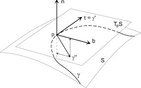
Consider a point $\mathrm{p} \in \mathcal{M}$. The set, $T_{\mathbf{p}}(\mathcal{M})$, of all vectors that are tangent to the manifold at the point $p$ forms a vector space called the tangent space at p. The tangent space has the same dimension as $\mathcal{M}$. Each tangent space $T_{\mathbf{p}}(\mathcal{M})$ at a point $\mathbf{p}$ has an inner-product, $g_{\mathbf{p}}=\langle\cdot, \cdot): T_{\mathbf{p}}(\mathcal{M}) \times T_{\mathbf{p}}(\mathcal{M}) \rightarrow \Re$, which is defined to vary smoothly over the manifold with $\mathbf{p}$. For $\mathbf{x}, \mathbf{y}, \mathbf{z} \in T_{\mathbf{p}}(\mathcal{M})$, the inner-product $g_{\mathbf{p}}$ is
bilinear: $g_{\mathbf{p}}(a \mathbf{x}+b \mathbf{y}, \mathbf{z})=a g_{\mathbf{p}}(\mathbf{x}, \mathbf{z})+b g_{\mathbf{p}}(\mathbf{y}, \mathbf{z})$, for $a, b \in \Re$,
symmetric: $g_{\mathbf{p}}(\mathbf{x}, \mathbf{y})=g_{\mathbf{p}}(\mathbf{y}, \mathbf{x})$,
positive-definite: $g_{\mathbf{p}}(\mathbf{x}, \mathbf{y}) \geq 0$ and $g_{\mathbf{p}}(\mathbf{x}, \mathbf{x})=0$ iff $\mathbf{x}=\mathbf{0}$.
The collection of inner-products $g=\left{g_{\mathbf{p}}: \mathbf{p} \in \mathcal{M}\right}$ is a Riemannian metric on $\mathcal{M}$, and the pair $(\mathcal{M}, g)$ defines a Riemannian manifold.
Suppose $\left(\mathcal{M}, g^{\mathcal{M}}\right)$ and $\left(\mathcal{N}, g^{\mathcal{N}}\right)$ are two Riemannian manifolds that have the same dimension, and let $\psi: \mathcal{M} \rightarrow \mathcal{N}$ be a diffeomorphism. Then, $\psi$ is an isometry if for all $\mathbf{p} \in \mathcal{M}$ and any two points $\mathbf{u}, \mathbf{v} \in T_{\mathbf{p}}(\mathcal{M}), g^{\mathcal{M}}(\mathbf{u}, \mathbf{v})=g^{\mathcal{N}}(\psi(\mathbf{u}), \psi(\mathbf{v}))$; in other words, $\psi$ is an isometry if $\psi$ “pulls back” one Riemannian metric to the other.
机器学习代写|流形学习代写manifold data learning代考|Curves and Geodesics
If the Riemannian manifold $(\mathcal{M}, g)$ is connected, it is a metric space with an induced topology that coincides with the underlying manifold topology. We can, therefore, define a function $d^{\mathcal{M}}$ on $\mathcal{M}$ that calculates distances between points on $\mathcal{M}$ and determines its structure.
Let $\mathbf{p}, \mathbf{q} \in \mathcal{M}$ be any two points on the Riemannian manifold $\mathcal{M}$. We first define the length of a (one-dimensional) curve in $\mathcal{M}$ that joins $\mathbf{p}$ to $\mathbf{q}$, and then the length of the shortest such curve.
A curve in $\mathcal{M}$ is defined as a smooth mapping from an open interval $\Lambda$ (which may have infinite length) in $\Re$ into $\mathcal{M}$. The point $\lambda \in \Lambda$ forms a parametrization of the curve. Let $c(\lambda)=\left(c_{1}(\lambda), \cdots, c_{d}(\lambda)\right)^{\tau}$ be a curve in $\Re^{d}$ parametrized by $\lambda \in \Lambda \subseteq \Re$. If we take the coordinate functions, $\left{c_{h}(\lambda)\right}$, of $c(\lambda)$ to be as smooth as needed (usually, $\mathcal{C}^{\infty}$, functions that have any number of continuous derivatives), then we say that $c$ is a smooth curve. If $c(\lambda+\alpha)=c(\lambda)$ for all $\lambda, \lambda+\alpha \in \Lambda$, the curve $c$ is said to be closed. The velocity (or tangent) vector at the point $\lambda$ is given by
$$
c^{\prime}(\lambda)=\left(c_{1}^{\prime}(\lambda), \cdots, c_{d}^{\prime}(\lambda)\right)^{\tau},
$$
where $c_{j}^{\prime}(\lambda)=d c_{j}(\lambda) / d \lambda$, and the “speed” of the curve is
$$
\left|c^{\prime}(\lambda)\right|=\left{\sum_{j=1}^{d}\left[c_{j}^{\prime}(\lambda)\right]^{2}\right}^{1 / 2} .
$$
Distance on a smooth curve $c$ is given by arc-length, which is measured from a fixed point $\lambda_{0}$ on that curve. Usually, the fixed point is taken to be the origin, $\lambda_{0}=0$, defined to be one of the two endpoints of the data. More generally, the arc-length $L(c)$ along the curve $c(\lambda)$ from point $\lambda_{0}$ to point $\lambda_{1}$ is defined as
$$
L(c)=\int_{\lambda_{0}}^{\lambda_{1}}\left|c^{\prime}(\lambda)\right| d \lambda
$$
In the event that a curve has unit speed, its arc-length is $L(c)=\lambda_{1}-\lambda_{0}$.
Example: The Unit Circle in $\Re^{2}$. The unit circle in $\Re^{2}$, which is defined as $\left{\left(x_{1}, x_{2}\right) \in \Re^{2}\right.$ : $\left.x_{1}^{2}+x_{2}^{2}=1\right}$, is a one-dimensional curve that can be parametrized as
$$
c(\lambda)=\left(c_{1}(\lambda), c_{2}(\lambda)\right)^{\tau}=(\cos \lambda, \sin \lambda)^{\top}, \quad \lambda \in[0,2 \pi)
$$
The unit circle is a closed curve, its velocity is $c^{\prime}(\lambda)=(-\sin \lambda, \cos \lambda)^{\tau}$, and its speed is $\left|c^{\prime}(\lambda)\right|=1$.
流形学习代写
机器学习代写|流形学习代写manifold data learning代考|Topological Manifolds
直到 1936 年,Hassler Whitney 才首次对抽象流形的性质进行了清晰的描述。我们将“流形”视为对曲面在三个维度上的更高维度的概括。拓扑空间米是维数的拓扑流形d(有时写为米d) 如果它是第二可数豪斯多夫空间,也是局部欧几里得的维数d. 最后一个条件是在流形上的每一点,都存在一个小的局部区域,使得流形具有欧几里得空间的性质。Hausdorff 条件确保流形上的不同点可以(通过邻域)分开,第二可数条件确保流形不会太大。Hausdorff 和第二可数性的两个条件,连同 Whitney (1936) 的嵌入定理,意味着任何d多维流形,米d, 可以嵌入R2d+1. 换句话说,最多一个空间2d+1尺寸需要嵌入d维流形。子流形只是位于另一个更高维度流形内的流形。作为拓扑空间,流形可以具有拓扑结构,例如紧凑或连通。
机器学习代写|流形学习代写manifold data learning代考|Riemannian Manifolds
在拓扑流形的整个理论中,没有提到微积分的使用。然而,在“流形”的原型应用中,微积分以“平滑”(或可微分)流形的形式出现米,也称为黎曼流形;它通常在微分几何中定义为一些周围(或周围)欧几里得空间的子流形,其中保留了长度、曲率和角度的概念,并且平滑度与可微性相关。Georg Friedrich Bernhard Riemann (1826-1866) 在他 1851 年的博士论文 (Riemann, 1851; Dieudonné, 2009) 中以“直观”的方式创造了流形这个词(德语,Mannigfaltigkeit),没有任何精确的定义;1854 年,黎曼在他著名的 Habrlitations 演讲中介绍了拓扑流形的概念,人们可以在该流形上进行微分和积分。
拓扑流形米称为光滑(或可微)流形,如果米连续可微分到任意阶。所有光滑流形都是拓扑流形,但反过来不一定正确。(注:作者经常对“平滑”流形的精确定义存在分歧。)
我们现在为可微流形定义同胚的类比。考虑两个开集,在∈ℜr和在∈ℜs, 然后让G:在→在所以对于X∈在和是∈在,G(X)= 是. 如果函数G具有有限的一阶偏导数,∂是j/∂X一世, 对全部一世=1,2,…,r, 和所有j=1,2,…,s, 然后G据说是一个平滑的(或可微的)映射在. 我们也说G是一个C1- 功能开启在如果所有一阶偏导数都是连续的。更一般地说,如果G具有连续的高阶偏导数,∂ķ1+⋯+ķr是j/∂X1ķ1⋯∂Xrķr, 对全部j=1,2,…,s和所有非负整数ķ1,ķ2,…,ķr这样ķ1+ķ2+⋯+ķr≤r,那么我们说G是一个C吨-功能,r=1,2,….如果G是一个Cr-所有人的功能r≥1,那么我们说G是一个C∞-功能。
如果G是开集的同胚在对开集在,则称其为Cr-微分同胚如果G和它的逆G−1都是Cr-职能。一种C∞-微分同胚简称为微分同胚。我们说在和在如果它们之间存在微分同胚,则它们是微分同胚的。这些定义以直接的方式扩展到流形。例如,如果X和是都是光滑流形,函数G:X→是如果它是同胚,则它是微分同胚X到是和两者G和G−1光滑。此外,X和是如果它们之间存在微分同胚,则它们是微分同胚的,在这种情况下,X和是本质上是无法区分的。
考虑一个点p∈米. 套装,吨p(米), 在该点与流形相切的所有向量p在 p 处形成一个称为切空间的向量空间。切线空间的维度与米. 每个切线空间吨p(米)在某一点p有一个内积,Gp=⟨⋅,⋅):吨p(米)×吨p(米)→ℜ, 它被定义为在流形上平滑变化p. 为了X,是,和∈吨p(米), 内积Gp是
双线性的:Gp(一种X+b是,和)=一种Gp(X,和)+bGp(是,和), 为了一种,b∈ℜ,
对称:Gp(X,是)=Gp(是,X),
正定:Gp(X,是)≥0和Gp(X,X)=0当且当X=0.
内积集合g=\left{g_{\mathbf{p}}: \mathbf{p} \in \mathcal{M}\right}g=\left{g_{\mathbf{p}}: \mathbf{p} \in \mathcal{M}\right}是黎曼度量米, 和对(米,G)定义了一个黎曼流形。
认为(米,G米)和(ñ,Gñ)是两个具有相同维度的黎曼流形,并且让ψ:米→ñ是微分同胚。然后,ψ如果对所有人来说是等距p∈米和任意两点在,在∈吨p(米),G米(在,在)=Gñ(ψ(在),ψ(在)); 换句话说,ψ是等距如果ψ将一个黎曼度量“拉回”到另一个。
机器学习代写|流形学习代写manifold data learning代考|Curves and Geodesics
如果黎曼流形(米,G)是连通的,它是一个度量空间,其诱导拓扑与底层流形拓扑一致。因此,我们可以定义一个函数d米在米计算点之间的距离米并确定其结构。
让p,q∈米是黎曼流形上的任意两点米. 我们首先定义一条(一维)曲线的长度米加入p到q,然后是最短的这种曲线的长度。
中的一条曲线米定义为开区间的平滑映射Λ(可能有无限长)在ℜ进入米. 重点λ∈Λ形成曲线的参数化。让C(λ)=(C1(λ),⋯,Cd(λ))τ成为曲线ℜd参数化λ∈Λ⊆ℜ. 如果我们取坐标函数,\left{c_{h}(\lambda)\right}\left{c_{h}(\lambda)\right}, 的C(λ)尽可能平滑(通常,C∞, 具有任意数量的连续导数的函数),那么我们说C是一条平滑曲线。如果C(λ+一种)=C(λ)对全部λ,λ+一种∈Λ, 曲线C据说是关闭的。该点的速度(或切线)矢量λ是(谁)给的
C′(λ)=(C1′(λ),⋯,Cd′(λ))τ,
在哪里Cj′(λ)=dCj(λ)/dλ,曲线的“速度”为
\left|c^{\prime}(\lambda)\right|=\left{\sum_{j=1}^{d}\left[c_{j}^{\prime}(\lambda)\right] ^{2}\right}^{1 / 2} 。\left|c^{\prime}(\lambda)\right|=\left{\sum_{j=1}^{d}\left[c_{j}^{\prime}(\lambda)\right] ^{2}\right}^{1 / 2} 。
平滑曲线上的距离C由弧长给出,从一个固定点测量λ0在那条曲线上。通常,以不动点为原点,λ0=0,定义为数据的两个端点之一。更一般地,弧长大号(C)沿着曲线C(λ)从点λ0指向λ1定义为
大号(C)=∫λ0λ1|C′(λ)|dλ
如果曲线具有单位速度,则其弧长为大号(C)=λ1−λ0.
示例:单位圆ℜ2. 单位圆在ℜ2, 定义为\left{\left(x_{1}, x_{2}\right) \in \Re^{2}\right.$ : $\left.x_{1}^{2}+x_{2}^{ 2}=1\右}\left{\left(x_{1}, x_{2}\right) \in \Re^{2}\right.$ : $\left.x_{1}^{2}+x_{2}^{ 2}=1\右}, 是一维曲线,可以参数化为
C(λ)=(C1(λ),C2(λ))τ=(因λ,罪λ)⊤,λ∈[0,2圆周率)
单位圆是一条闭合曲线,它的速度是C′(λ)=(−罪λ,因λ)τ, 它的速度是|C′(λ)|=1.

统计代写请认准statistics-lab™. statistics-lab™为您的留学生涯保驾护航。
金融工程代写
金融工程是使用数学技术来解决金融问题。金融工程使用计算机科学、统计学、经济学和应用数学领域的工具和知识来解决当前的金融问题,以及设计新的和创新的金融产品。
非参数统计代写
非参数统计指的是一种统计方法,其中不假设数据来自于由少数参数决定的规定模型;这种模型的例子包括正态分布模型和线性回归模型。
广义线性模型代考
广义线性模型(GLM)归属统计学领域,是一种应用灵活的线性回归模型。该模型允许因变量的偏差分布有除了正态分布之外的其它分布。
术语 广义线性模型(GLM)通常是指给定连续和/或分类预测因素的连续响应变量的常规线性回归模型。它包括多元线性回归,以及方差分析和方差分析(仅含固定效应)。
有限元方法代写
有限元方法(FEM)是一种流行的方法,用于数值解决工程和数学建模中出现的微分方程。典型的问题领域包括结构分析、传热、流体流动、质量运输和电磁势等传统领域。
有限元是一种通用的数值方法,用于解决两个或三个空间变量的偏微分方程(即一些边界值问题)。为了解决一个问题,有限元将一个大系统细分为更小、更简单的部分,称为有限元。这是通过在空间维度上的特定空间离散化来实现的,它是通过构建对象的网格来实现的:用于求解的数值域,它有有限数量的点。边界值问题的有限元方法表述最终导致一个代数方程组。该方法在域上对未知函数进行逼近。[1] 然后将模拟这些有限元的简单方程组合成一个更大的方程系统,以模拟整个问题。然后,有限元通过变化微积分使相关的误差函数最小化来逼近一个解决方案。
tatistics-lab作为专业的留学生服务机构,多年来已为美国、英国、加拿大、澳洲等留学热门地的学生提供专业的学术服务,包括但不限于Essay代写,Assignment代写,Dissertation代写,Report代写,小组作业代写,Proposal代写,Paper代写,Presentation代写,计算机作业代写,论文修改和润色,网课代做,exam代考等等。写作范围涵盖高中,本科,研究生等海外留学全阶段,辐射金融,经济学,会计学,审计学,管理学等全球99%专业科目。写作团队既有专业英语母语作者,也有海外名校硕博留学生,每位写作老师都拥有过硬的语言能力,专业的学科背景和学术写作经验。我们承诺100%原创,100%专业,100%准时,100%满意。
随机分析代写
随机微积分是数学的一个分支,对随机过程进行操作。它允许为随机过程的积分定义一个关于随机过程的一致的积分理论。这个领域是由日本数学家伊藤清在第二次世界大战期间创建并开始的。
时间序列分析代写
随机过程,是依赖于参数的一组随机变量的全体,参数通常是时间。 随机变量是随机现象的数量表现,其时间序列是一组按照时间发生先后顺序进行排列的数据点序列。通常一组时间序列的时间间隔为一恒定值(如1秒,5分钟,12小时,7天,1年),因此时间序列可以作为离散时间数据进行分析处理。研究时间序列数据的意义在于现实中,往往需要研究某个事物其随时间发展变化的规律。这就需要通过研究该事物过去发展的历史记录,以得到其自身发展的规律。
回归分析代写
多元回归分析渐进(Multiple Regression Analysis Asymptotics)属于计量经济学领域,主要是一种数学上的统计分析方法,可以分析复杂情况下各影响因素的数学关系,在自然科学、社会和经济学等多个领域内应用广泛。
MATLAB代写
MATLAB 是一种用于技术计算的高性能语言。它将计算、可视化和编程集成在一个易于使用的环境中,其中问题和解决方案以熟悉的数学符号表示。典型用途包括:数学和计算算法开发建模、仿真和原型制作数据分析、探索和可视化科学和工程图形应用程序开发,包括图形用户界面构建MATLAB 是一个交互式系统,其基本数据元素是一个不需要维度的数组。这使您可以解决许多技术计算问题,尤其是那些具有矩阵和向量公式的问题,而只需用 C 或 Fortran 等标量非交互式语言编写程序所需的时间的一小部分。MATLAB 名称代表矩阵实验室。MATLAB 最初的编写目的是提供对由 LINPACK 和 EISPACK 项目开发的矩阵软件的轻松访问,这两个项目共同代表了矩阵计算软件的最新技术。MATLAB 经过多年的发展,得到了许多用户的投入。在大学环境中,它是数学、工程和科学入门和高级课程的标准教学工具。在工业领域,MATLAB 是高效研究、开发和分析的首选工具。MATLAB 具有一系列称为工具箱的特定于应用程序的解决方案。对于大多数 MATLAB 用户来说非常重要,工具箱允许您学习和应用专业技术。工具箱是 MATLAB 函数(M 文件)的综合集合,可扩展 MATLAB 环境以解决特定类别的问题。可用工具箱的领域包括信号处理、控制系统、神经网络、模糊逻辑、小波、仿真等。