如果你也在 怎样代写多元统计分析Multivariate Statistical Analysis这个学科遇到相关的难题,请随时右上角联系我们的24/7代写客服。
多变量统计分析被认为是评估地球化学异常与任何单独变量和变量之间相互影响的意义的有用工具。
statistics-lab™ 为您的留学生涯保驾护航 在代写多元统计分析Multivariate Statistical Analysis方面已经树立了自己的口碑, 保证靠谱, 高质且原创的统计Statistics代写服务。我们的专家在代写多元统计分析Multivariate Statistical Analysis代写方面经验极为丰富,各种代写多元统计分析Multivariate Statistical Analysis相关的作业也就用不着说。
我们提供的多元统计分析Multivariate Statistical Analysis及其相关学科的代写,服务范围广, 其中包括但不限于:
- Statistical Inference 统计推断
- Statistical Computing 统计计算
- Advanced Probability Theory 高等概率论
- Advanced Mathematical Statistics 高等数理统计学
- (Generalized) Linear Models 广义线性模型
- Statistical Machine Learning 统计机器学习
- Longitudinal Data Analysis 纵向数据分析
- Foundations of Data Science 数据科学基础
统计代写|多元统计分析代写Multivariate Statistical Analysis代考|Discriminant Analysis
In discriminant analysis, we wish to decide which population an observation in a sample comes from, if the possible populations are known in advance. For example, suppose that we know in advance that some customers are “good” and some customers are “bad” (so the two possible populations, good customers and bad customers, are known in advance). Given a randomly selected customer, we wish to determine if he/she is a good customer or not based on his/her records (data) such as credit history $\left(x_{1}\right)$, education $\left(x_{2}\right)$, and income $\left(x_{3}\right)$. Such a discriminant analysis may be very useful for (say) credit card applicants so that good applicants will receive credit cards while bad applicants do not receive credit cards. For the convenience of statistical analysis, sometimes we may assume that the sample $\left(x_{1}, x_{2}, x_{3}\right)$ (or its transformations, e.g., $\left.\left(\log \left(x_{1}\right), \log \left(x_{2}\right), \log \left(x_{3}\right)\right)\right)$, follows a multivariate normal distribution, but some discriminant analysis methods do not require this assumption.
As another example, suppose that a company reviews job applicants based on their academic records $\left(x_{1}\right)$, education $\left(x_{2}\right)$, working experience $\left(x_{3}\right)$, self confidence $\left(x_{4}\right)$, and motivation $\left(x_{5}\right)$. All job applicants can be classified as either “suitable” or “not suitable” based on the given information. So the company may perform a discriminant analysis to separate suitable applicants from unsuitable applicants based on the data all applicants provide.
More generally, suppose that there are two multivariate normally distributed populations, denoted by
population $\pi_{1}: N_{p}\left(\boldsymbol{\mu}{1}, \Sigma{1}\right), \quad$ population $\pi_{2}: N_{p}\left(\boldsymbol{\mu}{2}, \Sigma{2}\right)$.
Given an observation $\mathrm{x}=\left(x_{1}, x_{2}, \cdots, x_{p}\right)^{\mathrm{T}}$ from a sample, we want to find out whether $\mathbf{x}$ is from population $\pi_{1}$ or population $\pi_{2}$. This is a discriminant analysis. Note that, if $p=1$ (i.e., if there is only one variable of interest), then it is very easy to separate the observations. All we need to do is to decide a threshold value, say $K$, so that we can do the separation based on whether $x \leqslant K$ or $x>K$. For example, if we just wish to separate students based on their grades, it is easy to see which students are good and which are not, such as the ones with grades over $80 \%$ and the ones with grades less than $80 \%$ (so $K=80$ ). However, when $p \geqslant 2$, it is less straightforward to separate the observations. For example, if we wish to separate students based on their grades and their music skills, then it may be hard to do the separation since a student may have very good grades but poor music skills. In this case, we need more advance statistical methods to do the separation.
There are many methods available for discriminant analysis. For example, the following two methods are simple and useful ones:
- Likelihood method: we may choose population $\pi_{1}$ if the likelihood for $\pi_{1}$ is larger
than the likelihood for $\pi_{2}$, or vice versa. This method requires distributional assumption, such as multivariate normal distributions.
- Mahalanobis distance method we may consider the Mahalanobis distances between an observation $\mathbf{x}$ and the population mean $\boldsymbol{\mu}{i}$ : $$ d{i}=\sqrt{\left(\mathrm{x}-\mu_{i}\right)^{\prime} \Sigma^{-1}\left(\mathrm{x}-\mu_{i}\right)}, \quad i=1,2,
$$
assuming $\Sigma_{1}=\Sigma_{2}=\Sigma$. We can then choose population $\pi_{1}$ if $d_{1}<d_{2}$, or vice versa. This method does not require distributional assumption.
统计代写|多元统计分析代写Multivariate Statistical Analysis代考|Discriminant analysis for categorical data
The discriminant analysis methods discussed so far assume that all the variables or data are continuous. When some variables or data are categorical or discrete, the above methods cannot be used since the means and covariance matrices are no longer meaningful for categorical variables or data. When some variables are categorical, a simple approach is to use logistic regression models for discriminant analysis, as illustrated below. Note that a logistic regression model is a generalized linear model, which will be described in details in Chapter 9 .
As an example, consider the case of two populations. Let $y=1$ if an observation $\mathbf{x}=\left(x_{1}, x_{2}, \cdots, x_{p}\right)^{\mathbf{T}}$ is from population 1 and $y=0$ if the observation is from population 2. Then, we can consider the following logistic regression model
$$
\log \frac{P(y=1)}{1-P(y=1)}=\beta_{0}+\beta_{1} x_{1}+\cdots+\beta_{p} x_{p},
$$
where some $x_{j}$ ‘s may be categorical and some may be continuous. Given data, the above logistic regression model can be used to fit the data. Then, we can estimate the probability $P(y=1)$ based on the fitted logistic regression model. For observation $\mathbf{x}{i}$, if the estimated probability $\widehat{P}\left(y{i}=1\right)>0.5$, observation $\mathbf{x}_{i}$ is more likely from population 1 ; otherwise it is more likely from population 2. This method can be extended to more than two populations.
统计代写|多元统计分析代写Multivariate Statistical Analysis代考|Cluster Analysis
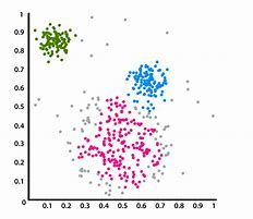
The goal of a cluster analysis is to identify homogeneous groups in the data by grouping observations based on their similarities or dis-similarities, i.e., similar observations are assigned to the same group. In other words, the idea is to partition all observations into subgroups or clusters (or populations), so that observations in the same cluster have similar characteristics.
For example, a marketing professional may want to partition all consumers into subgroups or clusters so that consumers in the same subgroup or cluster have similar buying habits. The partition can be based on age $\left(x_{1}\right)$, education $\left(x_{2}\right)$, income $\left(x_{3}\right)$, and monthly payments $\left(x_{4}\right)$. This is an example of cluster analysis based on four variables. The marketing professional may then design special advertisement strategies for different groups/clusters of consumers. Note that here the number of subgroups or clusters is not known before the cluster analysis.
Cluster analysis is similar to discriminant analysis in the sense that both methods try to separate observations into different groups. However, in discriminant analysis, the number of clusters (or subgroups or populations) are known in advance, and the objective is to determine which cluster (or population) an observation is likely to come from. In cluster analysis, on the other hand, the number of clusters (or subgroups or populations) is not known in advance, and the objective is find out distinct clusters and determine which cluster an observation is likely to come from. In other words, in cluster analysis one needs to find out how many clusters there may be and determine the cluster membership of an observation. Therefore, statistical methods for discriminant analysis may not be directly used in cluster analysis.
In cluster analysis, our objective is to devise a classification scheme, i.e., we need to find a rule to measure the similarity or dissimilarity between any two observations so that similar observations are grouped together to form clusters. Specifically, let $\mathbf{x}=\left(x_{1}, x_{2}, \cdots, x_{p}\right)^{\mathrm{T}}$ and $\mathbf{x}^{}=\left(x_{1}^{}, x_{2}^{}, \cdots, x_{p}^{}\right)^{\mathrm{T}}$ be two observations. The similarity between them can be measured by the “distance” between them, so that the two observations are similar if the distance between them is small. For example, the Euclidean distance between $\mathrm{x}$ and $\mathrm{x}^{}$ is defined as $$ d_{0}\left(\mathrm{x}, \mathrm{x}^{}\right)=\sqrt{\left(\mathrm{x}-\mathrm{x}^{}\right)^{\mathrm{T}}\left(\mathrm{x}-\mathrm{x}^{}\right)}=\sqrt{\sum_{j=1}^{p}\left(x_{j}-x_{j}^{}\right)^{2}} . $$ However, the Euclidean distance does not take into account the variations and the correlations of the component variables. For multivariate data, each individual component variable has its own variance and the component variables may be correlated. Therefore, a better measure of the “distance” between two multivariate observations $\mathbf{x}$ and $\mathbf{x}^{}$ is the Mahalanobis distance:
$$
d\left(\mathbf{x}, \mathbf{x}^{}\right)=\sqrt{\left(\mathbf{x}-\mathbf{x}^{}\right)^{\mathrm{T}} \Sigma^{-1}\left(\mathbf{x}-\mathbf{x}^{*}\right)}
$$
where $\Sigma=\operatorname{Cov}(\mathbf{x})=\operatorname{Cov}\left(\mathbf{x}^{}\right)$ is the covariance matrix, assuming the two observations have the same covariance matrices. Thus, if the distance $d\left(\mathbf{x}, \mathbf{x}^{}\right)$ is small, we can consider that $\mathrm{x}$ and $\mathrm{x}^{*}$ are “close” and put them in the same cluster/group. Otherwise, we can put them in different clusters/groups. For a sample of $n$ observations, $\left{\mathbf{x}{1}, \cdots, \mathbf{x}{n}\right}$, each observation can be assigned into one of the clusters, based on a clustering method.
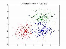
There are many cluster analysis methods available. In the following, we briefly discuss a few commonly used methods: nearest neighbour method, $k$-means algorithm, and two hierarchical cluster methods. Each method has its advantages and disadvantages, and different methods may lead to different results. In practice, it is always desirable to try at least two methods to analyze a dataset to see if the results agree or how much the results differ (which may provide some insights about the data).
多元统计分析代考
统计代写|多元统计分析代写Multivariate Statistical Analysis代考|Discriminant Analysis
在判别分析中,如果事先知道可能的总体,我们希望确定样本中的观察来自哪个总体。例如,假设我们预先知道有些客户是“好”,有些客户是“坏”(所以预先知道好客户和坏客户这两个可能的人群)。给定一个随机选择的客户,我们希望根据他/她的信用记录等记录(数据)来确定他/她是否是一个好客户(X1), 教育(X2), 和收入(X3). 这样的判别分析对于(比如说)信用卡申请者可能非常有用,因此好的申请者会收到信用卡,而坏的申请者不会收到信用卡。为方便统计分析,有时我们可以假设样本(X1,X2,X3)(或其转换,例如,(日志(X1),日志(X2),日志(X3))), 遵循多元正态分布,但一些判别分析方法不需要这个假设。
再举一个例子,假设一家公司根据求职者的学术记录来审查他们(X1), 教育(X2), 工作经验(X3), 自信心(X4), 和动机(X5). 根据给定的信息,所有求职者都可以分为“合适”或“不合适”。因此,公司可能会根据所有申请人提供的数据进行判别分析,将合适的申请人与不合适的申请人区分开来。
更一般地,假设有两个多元正态分布的总体,用
population表示圆周率1:ñp(μ1,Σ1),人口圆周率2:ñp(μ2,Σ2).
给定一个观察X=(X1,X2,⋯,Xp)吨从样本中,我们想知道是否X来自人口圆周率1或人口圆周率2. 这是判别分析。请注意,如果p=1(即,如果只有一个感兴趣的变量),那么很容易将观察结果分开。我们需要做的就是确定一个阈值,比如说ķ, 这样我们就可以根据是否X⩽ķ或者X>ķ. 例如,如果我们只是想根据成绩来区分学生,很容易看出哪些学生好哪些不好,比如成绩超过80%以及成绩低于80%(所以ķ=80)。然而,当p⩾2, 分开观察就不太容易了。例如,如果我们希望根据学生的成绩和音乐技能将学生分开,那么可能很难做到分开,因为学生可能成绩很好但音乐技能很差。在这种情况下,我们需要更先进的统计方法来进行分离。
有许多方法可用于判别分析。例如,以下两种方法是简单而有用的方法:
- 似然法:我们可以选择总体圆周率1如果可能性为圆周率1更大
比可能性圆周率2, 或相反亦然。此方法需要分布假设,例如多元正态分布。
- 马氏距离方法我们可以考虑观察之间的马氏距离X和人口平均μ一世 :d一世=(X−μ一世)′Σ−1(X−μ一世),一世=1,2,
假设Σ1=Σ2=Σ. 然后我们可以选择人口圆周率1如果d1<d2, 或相反亦然。这种方法不需要分布假设。
统计代写|多元统计分析代写Multivariate Statistical Analysis代考|Discriminant analysis for categorical data
到目前为止讨论的判别分析方法假设所有变量或数据都是连续的。当某些变量或数据是分类变量或离散数据时,不能使用上述方法,因为均值和协方差矩阵对分类变量或数据不再有意义。当某些变量是分类变量时,一种简单的方法是使用逻辑回归模型进行判别分析,如下图所示。请注意,逻辑回归模型是广义线性模型,将在第 9 章中详细介绍。
例如,考虑两个总体的情况。让是=1如果一个观察X=(X1,X2,⋯,Xp)吨来自人口 1 和是=0如果观察来自人口 2。那么,我们可以考虑以下逻辑回归模型
日志磷(是=1)1−磷(是=1)=b0+b1X1+⋯+bpXp,
其中一些Xj可能是分类的,有些可能是连续的。给定数据,上述逻辑回归模型可用于拟合数据。然后,我们可以估计概率磷(是=1)基于拟合的逻辑回归模型。用于观察X一世, 如果估计的概率磷^(是一世=1)>0.5, 观察X一世更有可能来自人口 1 ;否则更有可能来自种群 2。这种方法可以扩展到两个以上的种群。
统计代写|多元统计分析代写Multivariate Statistical Analysis代考|Cluster Analysis
聚类分析的目标是通过根据观察结果的相似性或不相似性对观察结果进行分组来识别数据中的同质组,即将相似的观察结果分配给同一组。换句话说,这个想法是将所有观测值划分为子组或集群(或总体),以便同一集群中的观测值具有相似的特征。
例如,营销专业人员可能希望将所有消费者划分为子组或集群,以便同一子组或集群中的消费者具有相似的购买习惯。分区可以基于年龄(X1), 教育(X2), 收入(X3), 和每月付款(X4). 这是一个基于四个变量的聚类分析示例。然后,营销专业人员可以为不同的消费者群体/集群设计特殊的广告策略。请注意,此处子组或聚类的数量在聚类分析之前是未知的。
聚类分析类似于判别分析,因为这两种方法都试图将观察结果分成不同的组。但是,在判别分析中,聚类(或子组或总体)的数量是预先知道的,目标是确定观察结果可能来自哪个聚类(或总体)。另一方面,在聚类分析中,事先不知道聚类(或子组或总体)的数量,目标是找出不同的聚类并确定观察结果可能来自哪个聚类。换句话说,在聚类分析中,需要找出可能有多少聚类并确定观察的聚类成员。因此,判别分析的统计方法可能不能直接用于聚类分析。
在聚类分析中,我们的目标是设计一个分类方案,即我们需要找到一个规则来衡量任何两个观测值之间的相似性或不相似性,以便将相似的观测值组合在一起形成聚类。具体来说,让X=(X1,X2,⋯,Xp)吨和X=(X1,X2,⋯,Xp)吨是两个观察。它们之间的相似性可以通过它们之间的“距离”来衡量,因此如果它们之间的距离很小,则两个观测值相似。例如,之间的欧几里得距离X和X定义为
d0(X,X)=(X−X)吨(X−X)=∑j=1p(Xj−Xj)2.然而,欧几里得距离没有考虑成分变量的变化和相关性。对于多变量数据,每个单独的组件变量都有自己的方差,并且组件变量可能是相关的。因此,更好地衡量两个多变量观测值之间的“距离”X和X是马氏距离:
d(X,X)=(X−X)吨Σ−1(X−X∗)
在哪里Σ=这(X)=这(X)是协方差矩阵,假设两个观测值具有相同的协方差矩阵。因此,如果距离d(X,X)很小,我们可以认为X和X∗是“关闭的”并将它们放在同一个集群/组中。否则,我们可以将它们放在不同的集群/组中。对于一个样本n观察,\left{\mathbf{x}{1}, \cdots, \mathbf{x}{n}\right}\left{\mathbf{x}{1}, \cdots, \mathbf{x}{n}\right},基于聚类方法,可以将每个观测值分配到其中一个聚类中。
有许多可用的聚类分析方法。下面,我们简要讨论几种常用的方法:最近邻法,ķ-means 算法和两种层次聚类方法。每种方法都有其优点和缺点,不同的方法可能导致不同的结果。在实践中,总是希望尝试至少两种方法来分析数据集,以查看结果是否一致或结果有多大差异(这可能会提供有关数据的一些见解)。

统计代写请认准statistics-lab™. statistics-lab™为您的留学生涯保驾护航。
金融工程代写
金融工程是使用数学技术来解决金融问题。金融工程使用计算机科学、统计学、经济学和应用数学领域的工具和知识来解决当前的金融问题,以及设计新的和创新的金融产品。
非参数统计代写
非参数统计指的是一种统计方法,其中不假设数据来自于由少数参数决定的规定模型;这种模型的例子包括正态分布模型和线性回归模型。
广义线性模型代考
广义线性模型(GLM)归属统计学领域,是一种应用灵活的线性回归模型。该模型允许因变量的偏差分布有除了正态分布之外的其它分布。
术语 广义线性模型(GLM)通常是指给定连续和/或分类预测因素的连续响应变量的常规线性回归模型。它包括多元线性回归,以及方差分析和方差分析(仅含固定效应)。
有限元方法代写
有限元方法(FEM)是一种流行的方法,用于数值解决工程和数学建模中出现的微分方程。典型的问题领域包括结构分析、传热、流体流动、质量运输和电磁势等传统领域。
有限元是一种通用的数值方法,用于解决两个或三个空间变量的偏微分方程(即一些边界值问题)。为了解决一个问题,有限元将一个大系统细分为更小、更简单的部分,称为有限元。这是通过在空间维度上的特定空间离散化来实现的,它是通过构建对象的网格来实现的:用于求解的数值域,它有有限数量的点。边界值问题的有限元方法表述最终导致一个代数方程组。该方法在域上对未知函数进行逼近。[1] 然后将模拟这些有限元的简单方程组合成一个更大的方程系统,以模拟整个问题。然后,有限元通过变化微积分使相关的误差函数最小化来逼近一个解决方案。
tatistics-lab作为专业的留学生服务机构,多年来已为美国、英国、加拿大、澳洲等留学热门地的学生提供专业的学术服务,包括但不限于Essay代写,Assignment代写,Dissertation代写,Report代写,小组作业代写,Proposal代写,Paper代写,Presentation代写,计算机作业代写,论文修改和润色,网课代做,exam代考等等。写作范围涵盖高中,本科,研究生等海外留学全阶段,辐射金融,经济学,会计学,审计学,管理学等全球99%专业科目。写作团队既有专业英语母语作者,也有海外名校硕博留学生,每位写作老师都拥有过硬的语言能力,专业的学科背景和学术写作经验。我们承诺100%原创,100%专业,100%准时,100%满意。
随机分析代写
随机微积分是数学的一个分支,对随机过程进行操作。它允许为随机过程的积分定义一个关于随机过程的一致的积分理论。这个领域是由日本数学家伊藤清在第二次世界大战期间创建并开始的。
时间序列分析代写
随机过程,是依赖于参数的一组随机变量的全体,参数通常是时间。 随机变量是随机现象的数量表现,其时间序列是一组按照时间发生先后顺序进行排列的数据点序列。通常一组时间序列的时间间隔为一恒定值(如1秒,5分钟,12小时,7天,1年),因此时间序列可以作为离散时间数据进行分析处理。研究时间序列数据的意义在于现实中,往往需要研究某个事物其随时间发展变化的规律。这就需要通过研究该事物过去发展的历史记录,以得到其自身发展的规律。
回归分析代写
多元回归分析渐进(Multiple Regression Analysis Asymptotics)属于计量经济学领域,主要是一种数学上的统计分析方法,可以分析复杂情况下各影响因素的数学关系,在自然科学、社会和经济学等多个领域内应用广泛。
MATLAB代写
MATLAB 是一种用于技术计算的高性能语言。它将计算、可视化和编程集成在一个易于使用的环境中,其中问题和解决方案以熟悉的数学符号表示。典型用途包括:数学和计算算法开发建模、仿真和原型制作数据分析、探索和可视化科学和工程图形应用程序开发,包括图形用户界面构建MATLAB 是一个交互式系统,其基本数据元素是一个不需要维度的数组。这使您可以解决许多技术计算问题,尤其是那些具有矩阵和向量公式的问题,而只需用 C 或 Fortran 等标量非交互式语言编写程序所需的时间的一小部分。MATLAB 名称代表矩阵实验室。MATLAB 最初的编写目的是提供对由 LINPACK 和 EISPACK 项目开发的矩阵软件的轻松访问,这两个项目共同代表了矩阵计算软件的最新技术。MATLAB 经过多年的发展,得到了许多用户的投入。在大学环境中,它是数学、工程和科学入门和高级课程的标准教学工具。在工业领域,MATLAB 是高效研究、开发和分析的首选工具。MATLAB 具有一系列称为工具箱的特定于应用程序的解决方案。对于大多数 MATLAB 用户来说非常重要,工具箱允许您学习和应用专业技术。工具箱是 MATLAB 函数(M 文件)的综合集合,可扩展 MATLAB 环境以解决特定类别的问题。可用工具箱的领域包括信号处理、控制系统、神经网络、模糊逻辑、小波、仿真等。