如果你也在 怎样代写实验设计experimental design这个学科遇到相关的难题,请随时右上角联系我们的24/7代写客服。
实验设计是一个概念,用于有效地组织、进行和解释实验结果,确保通过进行少量的试验获得尽可能多的有用信息。
statistics-lab™ 为您的留学生涯保驾护航 在代写实验设计experimental designatistical Modelling方面已经树立了自己的口碑, 保证靠谱, 高质且原创的统计Statistics代写服务。我们的专家在代写实验设计experimental design代写方面经验极为丰富,各种代写实验设计experimental design相关的作业也就用不着说。
我们提供的实验设计experimental design及其相关学科的代写,服务范围广, 其中包括但不限于:
- Statistical Inference 统计推断
- Statistical Computing 统计计算
- Advanced Probability Theory 高等楖率论
- Advanced Mathematical Statistics 高等数理统计学
- (Generalized) Linear Models 广义线性模型
- Statistical Machine Learning 统计机器学习
- Longitudinal Data Analysis 纵向数据分析
- Foundations of Data Science 数据科学基础
统计代写|实验设计作业代写experimental design代考|INTRODUCTION
When a model can be formed by including some, or all, of the predictor variables, there is a problem in deciding how many variables to include. The decision we arrive at will depend to some extent on the purpose we have in mind. If we merely wish to explain the variation of the dependent variable in the sample, then $1 \mathrm{t}$ would seem obvious that as many predictor variables as possible should be included. This can be seen with the lactation curve of Example $2.11$. If enough powers of $w$ were added to the model the curve would pass through every observed value, but it would be so jagged and complicated it would be difficult to understand what was happening. On the other hand, a small model has the advantage that it is easy to understand the relationships between the variables. Further more, a small model will usually yield estimators which are less influenced by peculiarites of the sample and so are more stable. Another important decision which must be made is whether to use the original predictor variables or to transform them in some way, often by taking a linear combination. For example, the cost of a particular kind of fencing for a rectangular field may largely depend on the length and breadth of the field. If all the fields in the
sample are in the same proportions then only one variable (length or breadth) would be needed. Even if they are not in the same proportions, one variable may be sufficient, namely the sum of the length and the breadth or, indeed, the perimeter. This is our ideal solution, reducing the number of predictor variables from two to one and at the same time obtaining a predictor variable which has physi= cal meaning, With a particular data set, the predicted value of the cost may be $y=1.11+0.9$ b so that the best single variable would be the $r$ ight hand side with $1=l$ ength and $b=b r e a d t h$, but this particular linear combination would have no physical meaning. We need to keep both aspects in mind, balancing statistioal optimum against physical meaning.
In the first section we shall 11 mit our discussion to orthogonal predictor variables, Although this may seem an unnecessarily strong restriction to place on the model, orthogonal variables of ten exist in experimental design situations. Indeed the values of the variables in the sample are often deliberately chosen to be orthogonal. We explain the advantages of this in section $3.2$, while in section $3.4$ we show that 1 t is possible to transform variables, for any data set, so that they are orthogonal.
统计代写|实验设计作业代写experimental design代考|ORTHOGONAL PREDICTOR VARIABLES
If the variables in a model are expressed as deviations from their means and if there are $k$ predictor variables, the sum of squares for regression is given by
$$
\begin{aligned}
\mathrm{SSR} &=b_{1} s_{y 1}+b_{2} s_{y 2}+\cdots+b_{k} s_{y k} \
&=s_{y 1}^{2} / s_{11}+s_{y 2}^{2} / s_{22}+\cdots+s_{y k}^{2} / s_{k k}
\end{aligned}
$$
The total sum of squares is
$$
\text { SST }-s_{y y}=\sum y_{i}^{2}
$$
By subtraction, we find the sum of squares for error (residual) is
$$
\mathrm{SSE}=S S T-S S R
$$
In this seotion, we assume that the predicton variables are orthog= onal and explore the implications of the number of variables included in the model.
We consider now the effect of adding another variable, $x_{k+1}$, to the model and assume that this variable $1 s$ also orthogonal to the other predfotor variables. The SST will not be affected by adding $x_{k+1}$ to the model. We introduce the notation that SSR(k) is the sum of squares for negression when the variables $x_{1}, x_{2}, \cdots x_{k}$ are in the model. It is clear that
(i) $\operatorname{SSR}(k+1) \geq \operatorname{SSR}(k)$
This follows from $(3.2 .1)$ as each term in the sum cannot be negative so that adding a further variable cannot decrease the sum of squares for regression.
(ii) $\operatorname{SSE}(k+1) \leq \operatorname{SSE}(k)$
This is the other side of the coin and follows from $(3.2 .2)$.
(111)
$$
R(k+1)^{2}=\operatorname{SSR}(k+1) / \operatorname{SST} \geq \mathrm{R}(k)^{2}=\operatorname{SSR}(k) / \mathrm{SST}
$$
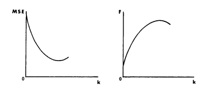
SSR $(k+1)$ can be thought of as the amount of variation in $y$ explained by the $(k+1)$ predictor variables, and $R(k+1)^{2}$ is the proportion of the variation in y explained by these variables. These monotone properties are illustrated by the diagrams in figure $3.2 .1$.
统计代写|实验设计作业代写experimental design代考|ADDING NONORTHOGONAL VARIABLES SEQUENTIALLY
Although orthogonal predictor variables are the ideal, they will rarely occur in practice with observational data. If some of the predictor variables are highly correlated, the matrix $X \mathrm{~T} X$ will be nearly singular. This could raise statistical and numerical problems, particularly if there is interest in estimating the coefficients of the model. We nave more to say on this in the next section and in a later section on Ridge Estimators.
Moderate correlations between predictor variables will cause few problems. While it is not essential to convert predictor variables to others which are orthogonal, it is instruotive to do so as it gives insight into the meaning of the coefficients and the tests of significance based on them.
In Problem 1.5, we considered predicting the outcome of a student in the mathematics paper 303 (which we denoted by y) by marks
recelved in the papers 201 and 203 (denoted by $x_{1}$ and $x_{2}$, respectively). The actual numbers of these papers are not relevant, but, for interest sake, the paper 201 was a calculus paper and 203 an al gebra paper, both at second year university level and 303 was a third year paper in algebra. The sum of squares for regression when $y$ is regressed singly and together on the $x$ variables (and the $F^{2}$ values) are:
$\begin{array}{lll}\text { SSR on } 201 \text { alone : } & 1433.6 & (.405) \ \text { SSR on } 203 \text { alone : } & 2129.2 & (.602) \ \text { SSR on } 201 \text { and } 203: & 2265.6 & (.641)\end{array}$
Clearly, the two $x$ variables are not orthogonal (and, in fact, the correlation coefficient between them is 0.622) as the individual sums of squares for regression do not add to that given by the model with both variables included. Once we have regressed the 303 marks on the 201 marks, the additional sum of squares due to $2031 \mathrm{~s}$ (2265.6 $1433.6)=832$. In this section we show how to adjust one variable for another so that they are orthogonal, and, as a consequence, their sums of squares for regression add to that given by the model with both variables included.
$\begin{array}{ll}\text { SSR for } 201 & =1433.6=\text { SSR for } x_{1} \ \text { SSR for } 203 \text { adjusted for } 201=832.0=\text { SSR for } z_{2} \ \text { SSR for } 201 \text { and } 203 & =2265.6\end{array}$
实验设计代考
统计代写|实验设计作业代写experimental design代考|INTRODUCTION
当可以通过包含一些或全部预测变量来形成模型时,在决定要包含多少变量时会出现问题。我们做出的决定在某种程度上取决于我们心中的目的。如果我们只是想解释样本中因变量的变化,那么1吨显然应该包括尽可能多的预测变量。这可以通过实施例的泌乳曲线看出2.11. 如果有足够的权力在被添加到模型中,曲线将通过每个观察值,但它会如此参差不齐和复杂,很难理解发生了什么。另一方面,小模型的优点是易于理解变量之间的关系。此外,小模型通常会产生受样本特性影响较小的估计量,因此更稳定。另一个必须做出的重要决定是是使用原始预测变量还是以某种方式转换它们,通常是通过线性组合。例如,矩形场地的特定类型围栏的成本可能在很大程度上取决于场地的长度和宽度。如果所有字段在
样本的比例相同,则只需要一个变量(长度或宽度)。即使它们的比例不同,一个变量可能就足够了,即长度和宽度的总和,或者实际上是周长。这是我们理想的解决方案,将预测变量的数量从两个减少到一个,同时得到一个具有物理意义的预测变量,对于特定的数据集,成本的预测值可能是是的=1.11+0.9b 这样最好的单一变量将是r右手边1=l长度和b=br和一种d吨H,但这种特殊的线性组合没有物理意义。我们需要牢记这两个方面,平衡统计优化与物理意义。
在第一节中,我们将讨论 11 到正交预测变量,尽管这似乎对模型施加了不必要的强限制,但在实验设计情况下存在 10 个正交变量。实际上,样本中变量的值通常被故意选择为正交的。我们在章节中解释了它的优点3.2, 而在截面3.4我们表明,对于任何数据集,1 t 都可以转换变量,使它们是正交的。
统计代写|实验设计作业代写experimental design代考|ORTHOGONAL PREDICTOR VARIABLES
如果模型中的变量表示为与其均值的偏差,并且如果存在ķ预测变量,回归的平方和由下式给出
小号小号R=b1s是的1+b2s是的2+⋯+bķs是的ķ =s是的12/s11+s是的22/s22+⋯+s是的ķ2/sķķ
总平方和为
SST −s是的是的=∑是的一世2
通过减法,我们发现误差(残差)的平方和为小号小号和=小号小号吨−小号小号R
在本节中,我们假设预测变量是正交的,并探讨模型中包含的变量数量的含义。
我们现在考虑添加另一个变量的效果,Xķ+1, 到模型并假设这个变量1s也与其他预测变量正交。SST 不会受到添加的影响Xķ+1到模型。我们引入符号 SSR(k) 是当变量X1,X2,⋯Xķ在模型中。很明显
(一)固态硬盘(ķ+1)≥固态硬盘(ķ)
这是从(3.2.1)因为总和中的每一项不能为负数,因此添加更多变量不能减少回归的平方和。
(二)上证所(ķ+1)≤上证所(ķ)
这是硬币的另一面,从(3.2.2).
(111)
R(ķ+1)2=固态硬盘(ķ+1)/SST≥R(ķ)2=固态硬盘(ķ)/小号小号吨
固态硬盘(ķ+1)可以认为是变化量是的由解释(ķ+1)预测变量,和R(ķ+1)2是这些变量解释的 y 变化的比例。这些单调特性由图中的图表说明3.2.1.
统计代写|实验设计作业代写experimental design代考|ADDING NONORTHOGONAL VARIABLES SEQUENTIALLY
尽管正交预测变量是理想的,但它们在实际观测数据中很少出现。如果某些预测变量高度相关,则矩阵X 吨X几乎是单数。这可能会引发统计和数值问题,特别是如果有兴趣估计模型的系数。我们将在下一节和后面关于岭估计器的部分中对此进行更多说明。
预测变量之间的中等相关性将导致很少的问题。虽然将预测变量转换为其他正交变量并不是必需的,但这样做具有指导意义,因为它可以深入了解系数的含义以及基于它们的显着性检验。
在问题 1.5 中,我们考虑用分数来预测学生在数学试卷 303(我们用 y 表示)中的结果
在 201 和 203 号论文中得到认可(记为X1和X2, 分别)。这些论文的实际数量无关紧要,但出于兴趣,论文 201 是微积分论文,203 是代数论文,都是大学二年级的论文,303 是代数三年级的论文。回归时的平方和是的在X变量(和F2值)是:
SSR 开启 201 独自的 : 1433.6(.405) SSR 开启 203 独自的 : 2129.2(.602) SSR 开启 201 和 203:2265.6(.641)
很明显,两人X变量不是正交的(实际上,它们之间的相关系数为 0.622),因为回归的各个平方和不会添加到包含两个变量的模型给出的平方和。一旦我们在 201 分上回归了 303 分,额外的平方和由于2031 s (2265.6 1433.6)=832. 在本节中,我们将展示如何将一个变量调整为另一个变量,以使它们正交,因此,它们的回归平方和与包含两个变量的模型给出的平方和相加。
SSR 为 201=1433.6= SSR 为 X1 SSR 为 203 调整为 201=832.0= SSR 为 和2 SSR 为 201 和 203=2265.6

统计代写请认准statistics-lab™. statistics-lab™为您的留学生涯保驾护航。
金融工程代写
金融工程是使用数学技术来解决金融问题。金融工程使用计算机科学、统计学、经济学和应用数学领域的工具和知识来解决当前的金融问题,以及设计新的和创新的金融产品。
非参数统计代写
非参数统计指的是一种统计方法,其中不假设数据来自于由少数参数决定的规定模型;这种模型的例子包括正态分布模型和线性回归模型。
广义线性模型代考
广义线性模型(GLM)归属统计学领域,是一种应用灵活的线性回归模型。该模型允许因变量的偏差分布有除了正态分布之外的其它分布。
术语 广义线性模型(GLM)通常是指给定连续和/或分类预测因素的连续响应变量的常规线性回归模型。它包括多元线性回归,以及方差分析和方差分析(仅含固定效应)。
有限元方法代写
有限元方法(FEM)是一种流行的方法,用于数值解决工程和数学建模中出现的微分方程。典型的问题领域包括结构分析、传热、流体流动、质量运输和电磁势等传统领域。
有限元是一种通用的数值方法,用于解决两个或三个空间变量的偏微分方程(即一些边界值问题)。为了解决一个问题,有限元将一个大系统细分为更小、更简单的部分,称为有限元。这是通过在空间维度上的特定空间离散化来实现的,它是通过构建对象的网格来实现的:用于求解的数值域,它有有限数量的点。边界值问题的有限元方法表述最终导致一个代数方程组。该方法在域上对未知函数进行逼近。[1] 然后将模拟这些有限元的简单方程组合成一个更大的方程系统,以模拟整个问题。然后,有限元通过变化微积分使相关的误差函数最小化来逼近一个解决方案。
tatistics-lab作为专业的留学生服务机构,多年来已为美国、英国、加拿大、澳洲等留学热门地的学生提供专业的学术服务,包括但不限于Essay代写,Assignment代写,Dissertation代写,Report代写,小组作业代写,Proposal代写,Paper代写,Presentation代写,计算机作业代写,论文修改和润色,网课代做,exam代考等等。写作范围涵盖高中,本科,研究生等海外留学全阶段,辐射金融,经济学,会计学,审计学,管理学等全球99%专业科目。写作团队既有专业英语母语作者,也有海外名校硕博留学生,每位写作老师都拥有过硬的语言能力,专业的学科背景和学术写作经验。我们承诺100%原创,100%专业,100%准时,100%满意。
随机分析代写
随机微积分是数学的一个分支,对随机过程进行操作。它允许为随机过程的积分定义一个关于随机过程的一致的积分理论。这个领域是由日本数学家伊藤清在第二次世界大战期间创建并开始的。
时间序列分析代写
随机过程,是依赖于参数的一组随机变量的全体,参数通常是时间。 随机变量是随机现象的数量表现,其时间序列是一组按照时间发生先后顺序进行排列的数据点序列。通常一组时间序列的时间间隔为一恒定值(如1秒,5分钟,12小时,7天,1年),因此时间序列可以作为离散时间数据进行分析处理。研究时间序列数据的意义在于现实中,往往需要研究某个事物其随时间发展变化的规律。这就需要通过研究该事物过去发展的历史记录,以得到其自身发展的规律。
回归分析代写
多元回归分析渐进(Multiple Regression Analysis Asymptotics)属于计量经济学领域,主要是一种数学上的统计分析方法,可以分析复杂情况下各影响因素的数学关系,在自然科学、社会和经济学等多个领域内应用广泛。
MATLAB代写
MATLAB 是一种用于技术计算的高性能语言。它将计算、可视化和编程集成在一个易于使用的环境中,其中问题和解决方案以熟悉的数学符号表示。典型用途包括:数学和计算算法开发建模、仿真和原型制作数据分析、探索和可视化科学和工程图形应用程序开发,包括图形用户界面构建MATLAB 是一个交互式系统,其基本数据元素是一个不需要维度的数组。这使您可以解决许多技术计算问题,尤其是那些具有矩阵和向量公式的问题,而只需用 C 或 Fortran 等标量非交互式语言编写程序所需的时间的一小部分。MATLAB 名称代表矩阵实验室。MATLAB 最初的编写目的是提供对由 LINPACK 和 EISPACK 项目开发的矩阵软件的轻松访问,这两个项目共同代表了矩阵计算软件的最新技术。MATLAB 经过多年的发展,得到了许多用户的投入。在大学环境中,它是数学、工程和科学入门和高级课程的标准教学工具。在工业领域,MATLAB 是高效研究、开发和分析的首选工具。MATLAB 具有一系列称为工具箱的特定于应用程序的解决方案。对于大多数 MATLAB 用户来说非常重要,工具箱允许您学习和应用专业技术。工具箱是 MATLAB 函数(M 文件)的综合集合,可扩展 MATLAB 环境以解决特定类别的问题。可用工具箱的领域包括信号处理、控制系统、神经网络、模糊逻辑、小波、仿真等。