如果你也在 怎样代写贝叶斯分析Bayesian Analysis这个学科遇到相关的难题,请随时右上角联系我们的24/7代写客服。
贝叶斯分析,一种统计推断方法(以英国数学家托马斯-贝叶斯命名),允许人们将关于人口参数的先验信息与样本所含信息的证据相结合,以指导统计推断过程。
statistics-lab™ 为您的留学生涯保驾护航 在代写贝叶斯分析Bayesian Analysis方面已经树立了自己的口碑, 保证靠谱, 高质且原创的统计Statistics代写服务。我们的专家在代写贝叶斯分析Bayesian Analysis代写方面经验极为丰富,各种代写贝叶斯分析Bayesian Analysis相关的作业也就用不着说。
我们提供的贝叶斯分析Bayesian Analysis及其相关学科的代写,服务范围广, 其中包括但不限于:
- Statistical Inference 统计推断
- Statistical Computing 统计计算
- Advanced Probability Theory 高等概率论
- Advanced Mathematical Statistics 高等数理统计学
- (Generalized) Linear Models 广义线性模型
- Statistical Machine Learning 统计机器学习
- Longitudinal Data Analysis 纵向数据分析
- Foundations of Data Science 数据科学基础
统计代写|贝叶斯分析代写Bayesian Analysis代考|Time Series and Regression
The first time series to be presented is the linear regression model with AR (1) errors, where $\mathrm{R}$ is employed to generate observations from that linear model with known parameters followed by an execution with WinBUGS that produces point and interval estimates of those parameters. The scenario is repeated for a quadratic regression with seasonal effects and AR(1) errors. In all scenarios, $R$ code generates the data and using that as information for the Bayesian analysis, the posterior distribution of the parameters is easily provided. Various generalizations to more complicated situations include a nonlinear regression model (with exponential trend) with AR(1) errors, a linear regression model with AR(2) errors which contains five parameters, two linear regression coefficients, two autoregressive parameters, plus the precision of the error terms. An interesting time series model is one which is continuous time, which is the solution to a stochastic differential equation, where the posterior distribution of the autoregressive parameter is derived assuming a noninformative prior distribution for the autoregressive parameter and the variance of the errors. The chapter concludes with a section on comments and conclusions followed by eight problems and eight references.
统计代写|贝叶斯分析代写Bayesian Analysis代考|Time Series and Stationarity
Stationarity of a time series is defined including stationary in the mean and stationary in the variance. The first time series to be considered is the moving average model and the first and second moments are derived. It is important to note that moving average processes are always stationary. $R$ is employed to generate observations from an MA(1) series with known parameters (the moving average coefficient and the precision of the white noise); then using those observations, WinBUGS is executed for the posterior analysis which provides point and credible intervals for the two parameters. The MA(1) series is generalized to quadratic regression model with MA(1) errors, where again $\mathrm{R}$ generates observations from it where the parameters are known.
Bayesian analysis via WinBUGS performs the posterior analysis. An additional generalization focuses on a quadratic regression model with an MA(2) series for the errors with $R$ used to generate observations from the model but with known values for the parameters. It is interesting to compare the results of the posterior estimates of the quadratic regression with MA(1) errors to that with MA(1) errors. Generalizing to a regression model with a quadratic trend, but also including seasonal effects, presents a challenge to the Bayesian way of determining the posterior analysis. The predictive density for forecasting future observations is derived, and the last section of the chapter presents the Bayesian technique of testing hypotheses about the moving average parameters. There are 16 exercises and 5 references.
统计代写|贝叶斯分析代写Bayesian Analysis代考|Time Series and Spectral Analysis
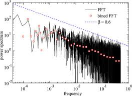
It is explained how spectral analysis gives an alternative approach to studying time series, where the emphasis is on the frequency of the series, instead of the time. Chapter 7 continues with a brief history of the role of the spectral density function in time series analysis, and the review includes an introduction to time series with trigonometric components (sine and cosine functions) as independent variables. Next to be explained are time series with trigonometric components whose coefficients are Fourier frequencies and their posterior distributions are revealed with a Bayesian analysis. It is important to remember that frequency is measured in hertz (one cycle per second) or in periods measured as so many units of pi radians per unit time. It can be shown that for the basic time series (autoregressive and moving average series), the spectral density function is known in terms of the parameters of the corresponding model. It is important to remember the spectrum is related to the Fourier line spectrum which is a plot of the fundamental frequencies versus $m$, where $m$ is the number of harmonics in the series. Section 10 continues with the derivation of the spectral density function for the basic series, AR(1), AR (2), MA(1), MA(2), ARMA(1,1), etc. Remember that the spectral density function is a function of frequency (measured in hertz or multiples of $\mathrm{pi}$ in radians per cycle). For each model, $\mathrm{R}$ is used to generate observations from that model (with known parameters); then, using those observations as data, the Bayesian analysis is executed with WinBUGS and as a consequence the posterior distribution of the spectral density at various frequencies is estimated. For the last example, the spectral density of the sunspot cycle is estimated via a Bayesian analysis executed with WinBUGS. There are 17 problems followed by $y$ references.
贝叶斯分析代考
统计代写|贝叶斯分析代写Bayesian Analysis代考|Time Series and Regression
要呈现的第一个时间序列是具有 AR (1) 误差的线性回归模型,其中R用于从具有已知参数的线性模型生成观察结果,然后使用 WinBUGS 执行生成这些参数的点和区间估计。对具有季节性影响和 AR(1) 误差的二次回归重复该场景。在所有场景中,R代码生成数据并将其用作贝叶斯分析的信息,很容易提供参数的后验分布。对更复杂情况的各种推广包括具有 AR(1) 误差的非线性回归模型(具有指数趋势)、具有 AR(2) 误差的线性回归模型,其中包含五个参数、两个线性回归系数、两个自回归参数以及精度的错误条款。一个有趣的时间序列模型是连续时间模型,它是随机微分方程的解,其中自回归参数的后验分布是在假设自回归参数和误差方差的非信息性先验分布的情况下导出的。
统计代写|贝叶斯分析代写Bayesian Analysis代考|Time Series and Stationarity
定义时间序列的平稳性,包括均值平稳和方差平稳。要考虑的第一个时间序列是移动平均模型,并推导出一阶矩和二阶矩。重要的是要注意,移动平均过程始终是静止的。R用于从具有已知参数(移动平均系数和白噪声精度)的 MA(1) 系列生成观测值;然后使用这些观察结果,执行 WinBUGS 进行后验分析,为两个参数提供点和可信区间。MA(1) 系列被推广到具有 MA(1) 误差的二次回归模型,其中再次R在参数已知的情况下从中生成观察结果。
通过 WinBUGS 进行的贝叶斯分析执行后验分析。另一个概括侧重于具有 MA(2) 系列的二次回归模型,其误差为R用于从模型生成观测值,但参数值已知。将具有 MA(1) 误差的二次回归的后验估计结果与具有 MA(1) 误差的结果进行比较是很有趣的。推广到具有二次趋势但也包括季节性影响的回归模型,对确定后验分析的贝叶斯方法提出了挑战。推导出预测未来观测的预测密度,本章的最后一节介绍了检验有关移动平均参数的假设的贝叶斯技术。有16个练习和5个参考。
统计代写|贝叶斯分析代写Bayesian Analysis代考|Time Series and Spectral Analysis
解释了频谱分析如何为研究时间序列提供了另一种方法,其中重点是序列的频率,而不是时间。第 7 章继续简要介绍了谱密度函数在时间序列分析中的作用,并介绍了以三角分量(正弦和余弦函数)作为自变量的时间序列。接下来要解释的是具有三角分量的时间序列,其系数是傅立叶频率,并且它们的后验分布通过贝叶斯分析来揭示。重要的是要记住,频率以赫兹(每秒一个周期)或以每单位时间 pi 弧度为单位的周期测量。可以证明,对于基本时间序列(自回归和移动平均序列),谱密度函数根据相应模型的参数是已知的。重要的是要记住频谱与傅里叶线谱有关,这是基本频率与米, 在哪里米是系列中的谐波数。第 10 节继续推导基本序列 AR(1)、AR(2)、MA(1)、MA(2)、ARMA(1,1) 等的谱密度函数。请记住,谱密度函数是频率的函数(以赫兹或p一世以弧度/周期为单位)。对于每个模型,R用于从该模型生成观测值(具有已知参数);然后,使用这些观察结果作为数据,使用 WinBUGS 执行贝叶斯分析,从而估计各种频率的谱密度的后验分布。对于最后一个示例,太阳黑子周期的光谱密度是通过使用 WinBUGS 执行的贝叶斯分析来估计的。后面有17个问题是参考。

统计代写请认准statistics-lab™. statistics-lab™为您的留学生涯保驾护航。
金融工程代写
金融工程是使用数学技术来解决金融问题。金融工程使用计算机科学、统计学、经济学和应用数学领域的工具和知识来解决当前的金融问题,以及设计新的和创新的金融产品。
非参数统计代写
非参数统计指的是一种统计方法,其中不假设数据来自于由少数参数决定的规定模型;这种模型的例子包括正态分布模型和线性回归模型。
广义线性模型代考
广义线性模型(GLM)归属统计学领域,是一种应用灵活的线性回归模型。该模型允许因变量的偏差分布有除了正态分布之外的其它分布。
术语 广义线性模型(GLM)通常是指给定连续和/或分类预测因素的连续响应变量的常规线性回归模型。它包括多元线性回归,以及方差分析和方差分析(仅含固定效应)。
有限元方法代写
有限元方法(FEM)是一种流行的方法,用于数值解决工程和数学建模中出现的微分方程。典型的问题领域包括结构分析、传热、流体流动、质量运输和电磁势等传统领域。
有限元是一种通用的数值方法,用于解决两个或三个空间变量的偏微分方程(即一些边界值问题)。为了解决一个问题,有限元将一个大系统细分为更小、更简单的部分,称为有限元。这是通过在空间维度上的特定空间离散化来实现的,它是通过构建对象的网格来实现的:用于求解的数值域,它有有限数量的点。边界值问题的有限元方法表述最终导致一个代数方程组。该方法在域上对未知函数进行逼近。[1] 然后将模拟这些有限元的简单方程组合成一个更大的方程系统,以模拟整个问题。然后,有限元通过变化微积分使相关的误差函数最小化来逼近一个解决方案。
tatistics-lab作为专业的留学生服务机构,多年来已为美国、英国、加拿大、澳洲等留学热门地的学生提供专业的学术服务,包括但不限于Essay代写,Assignment代写,Dissertation代写,Report代写,小组作业代写,Proposal代写,Paper代写,Presentation代写,计算机作业代写,论文修改和润色,网课代做,exam代考等等。写作范围涵盖高中,本科,研究生等海外留学全阶段,辐射金融,经济学,会计学,审计学,管理学等全球99%专业科目。写作团队既有专业英语母语作者,也有海外名校硕博留学生,每位写作老师都拥有过硬的语言能力,专业的学科背景和学术写作经验。我们承诺100%原创,100%专业,100%准时,100%满意。
随机分析代写
随机微积分是数学的一个分支,对随机过程进行操作。它允许为随机过程的积分定义一个关于随机过程的一致的积分理论。这个领域是由日本数学家伊藤清在第二次世界大战期间创建并开始的。
时间序列分析代写
随机过程,是依赖于参数的一组随机变量的全体,参数通常是时间。 随机变量是随机现象的数量表现,其时间序列是一组按照时间发生先后顺序进行排列的数据点序列。通常一组时间序列的时间间隔为一恒定值(如1秒,5分钟,12小时,7天,1年),因此时间序列可以作为离散时间数据进行分析处理。研究时间序列数据的意义在于现实中,往往需要研究某个事物其随时间发展变化的规律。这就需要通过研究该事物过去发展的历史记录,以得到其自身发展的规律。
回归分析代写
多元回归分析渐进(Multiple Regression Analysis Asymptotics)属于计量经济学领域,主要是一种数学上的统计分析方法,可以分析复杂情况下各影响因素的数学关系,在自然科学、社会和经济学等多个领域内应用广泛。
MATLAB代写
MATLAB 是一种用于技术计算的高性能语言。它将计算、可视化和编程集成在一个易于使用的环境中,其中问题和解决方案以熟悉的数学符号表示。典型用途包括:数学和计算算法开发建模、仿真和原型制作数据分析、探索和可视化科学和工程图形应用程序开发,包括图形用户界面构建MATLAB 是一个交互式系统,其基本数据元素是一个不需要维度的数组。这使您可以解决许多技术计算问题,尤其是那些具有矩阵和向量公式的问题,而只需用 C 或 Fortran 等标量非交互式语言编写程序所需的时间的一小部分。MATLAB 名称代表矩阵实验室。MATLAB 最初的编写目的是提供对由 LINPACK 和 EISPACK 项目开发的矩阵软件的轻松访问,这两个项目共同代表了矩阵计算软件的最新技术。MATLAB 经过多年的发展,得到了许多用户的投入。在大学环境中,它是数学、工程和科学入门和高级课程的标准教学工具。在工业领域,MATLAB 是高效研究、开发和分析的首选工具。MATLAB 具有一系列称为工具箱的特定于应用程序的解决方案。对于大多数 MATLAB 用户来说非常重要,工具箱允许您学习和应用专业技术。工具箱是 MATLAB 函数(M 文件)的综合集合,可扩展 MATLAB 环境以解决特定类别的问题。可用工具箱的领域包括信号处理、控制系统、神经网络、模糊逻辑、小波、仿真等。