如果你也在 怎样代写r语言这个学科遇到相关的难题,请随时右上角联系我们的24/7代写客服。
R是一种用于统计计算和图形的编程语言,由R核心团队和R统计计算基金会支持。R由统计学家Ross Ihaka和Robert Gentleman创建,在数据挖掘者和统计学家中被用于数据分析和开发统计软件。用户已经创建了软件包来增强R语言的功能。
根据用户调查和对学术文献数据库的研究,R是数据挖掘中最常用的编程语言之一。[6] 截至2022年3月,R在衡量编程语言普及程度的TIOBE指数中排名第11位。
官方的R软件环境是GNU软件包中的一个开源自由软件环境,在GNU通用公共许可证下提供。它主要是用C、Fortran和R本身(部分自我托管)编写的。预编译的可执行文件提供给各种操作系统。R有一个命令行界面。[8] 也有多个第三方图形用户界面,如RStudio,一个集成开发环境,和Jupyter,一个笔记本界面。
statistics-lab™ 为您的留学生涯保驾护航 在代写r语言方面已经树立了自己的口碑, 保证靠谱, 高质且原创的统计Statistics代写服务。我们的专家在代写r语言代写方面经验极为丰富,各种代写r语言相关的作业也就用不着说。
我们提供的r语言及其相关学科的代写,服务范围广, 其中包括但不限于:
- Statistical Inference 统计推断
- Statistical Computing 统计计算
- Advanced Probability Theory 高等楖率论
- Advanced Mathematical Statistics 高等数理统计学
- (Generalized) Linear Models 广义线性模型
- Statistical Machine Learning 统计机器学习
- Longitudinal Data Analysis 纵向数据分析
- Foundations of Data Science 数据科学基础
统计代写|r语言作业代写代考|Converting Daily Prices to Monthly Returns with tibbletime
This is a good time to introduce the relatively new tibbletime package, which is purpose-built for working with time-aware tibbles. In the flow below, we will first convert prices to a tibble with tk_tbl(). Then, we convert to a tibbletime object with a as_tbl_time(index = date) and then convert to monthly prices with as_period(period = “month”, side = “end”). The side argument anchors to the end of the month instead of the beginning. Try changing it to side = “start”.
This flow might not seem efficient – going from xts to tibble to tibbletime – but in future chapters we will see that rolling functions are smoother with rollify () and we can absorb some inefficiency now for future gains. Plus, the package is new and its capabilities are growing fast.
Before we move on, a quick review of our 4 monthly log return objects:
First, look at the date in each object. asset_returns_xts has a date index, not a column. That index does not have a name. It is accessed via index(asset_returns_xts).
The tibbles have a column called “date”, accessed via the \$date convention, e.g. asset_returns_dplyr_byhand\$date. That distinction is not important when we read with our eyes, but it is very important when we pass these objects to functions.
Second, each of these objects is in “wide” format, which in this case means there is a column for each of our assets: SPY has a column, EFA has a column, IJS has a column, EEM has a column, AGG has a column.
This is the format that xts likes and this format is easier for a human to read. However, the tidyverse calls for this data to be in long or tidy format where each variable has its own column. For asset returns to be tidy, we need a column called “date”, a column called “asset” and a column called “returns”.
To see that in action, here is how it looks.
统计代写|r语言作业代写代考|Visualizing Asset Returns in the xts world
It might seem odd that visualization is part of the data import and wrangling work flow and it does not have to be: we could jump straight into the process of converting these assets into a portfolio. However, it is a good practice to chart individual returns because once a portfolio is built, we are unlikely to
back track to visualizing on an individual basis. Yet, those individual returns are the building blocks and raw material of our portfolio and visualizing them is a great way to understand them deeply. It also presents an opportunity to look for outliers, or errors, or anything unusual to be corrected before we move too far along in our analysis.
For the purposes of visualizing returns, we will work with two of our monthly log returns objects, asset_returns_xts and asset_returns_long (the tidy, long-formatted tibble).
We start with the highcharter package to visualize the xts formatted returns.
highcharter is an $\mathrm{R}$ package but Highcharts is a JavaScript library. The $\mathrm{R}$ package is a hook into the JavaScript library. Highcharts is fantastic for visualizing time series and it comes with great built-in widgets for viewing different time frames, plus we get to use the power of JavaScript without leaving the world of $R$ code.
Not only are the visualizations nice, but highcharter “just works” with xts objects in the sense that it reads the index as dates without needing to be told. We pass in an xts object and let the package do the rest. I highly recommend it for visualizing financial time series but you do need to buy a license for use in a commercial setting. ${ }^{1}$
Let’s see how it works for charting our asset monthly returns.
统计代写|r语言作业代写代考|Visualizing Asset Returns in the tidyverse
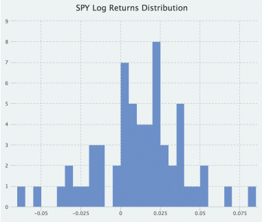
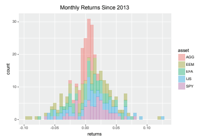
ggplot2 is a very widely-used and flexible visualization package, and it is part of the tidyverse. We will use it to build a histogram and have our first look at how tidy data plays nicely with functions in the tidyverse.
In the code chunk below, we start with our tidy object of returns, asset_returns_long, and then pipe to ggplot() with the $\%>\%$ operator. Next, we call ggplot (aes $(x=$ returns, $f i l 1=$ asset $)$ ) to indicate that returns will be on the $\mathrm{x}$-axis and that the bars should be filled with a different color for each asset. If we were to stop here, ggplot() would build an empty chart and that is because we have told it that we want a chart with certain
$\mathrm{x}$-axis values, but we have not told it what kind of chart to build. In ggplot() parlance, we have not yet specified a geom.
We use geom_histogram() to build a histogram and that means we do not specify a $y$-axis value, because the histogram will be based on counts of the returns.
Because the data frame is tidy and grouped by the asset column (recall when it was built we called group_by (asset)), ggplot() knows to chart a separate histogram for each asset. ggplot() will automatically include a legend since we included fill = asset in the aes () call.
R语言代写
统计代写|r语言作业代写代考|Converting Daily Prices to Monthly Returns with tibbletime
现在是介绍相对较新的 tibbletime 包的好时机,它是专门为处理时间感知 tibble 而构建的。在下面的流程中,我们将首先使用 tk_tbl() 将价格转换为 tibble。然后,我们使用 as_tbl_time(index = date) 转换为 tibbletime 对象,然后使用 as_period(period = “month”, side = “end”) 转换为月度价格。side 参数锚定到月底而不是月初。尝试将其更改为 side = “start”。
这个流程可能看起来效率不高——从 xts 到 tibble 再到 tibbletime——但在以后的章节中,我们将看到滚动函数使用 rollify() 更加平滑,我们现在可以吸收一些低效率以获得未来收益。此外,该软件包是新的,其功能正在快速增长。
在我们继续之前,快速回顾一下我们的 4 个月日志返回对象:
首先,查看每个对象中的日期。asset_returns_xts 有一个日期索引,而不是一个列。该索引没有名称。它通过 index(asset_returns_xts) 访问。
小标题有一个名为“date”的列,通过$ date 约定访问,例如asset_returns_dplyr_byhand $ date。当我们用肉眼阅读时,这种区别并不重要,但当我们将这些对象传递给函数时,它却非常重要。
其次,这些对象中的每一个都是“宽”格式,在这种情况下,这意味着我们的每个资产都有一个列:SPY 有一个列,EFA 有一个列,IJS 有一个列,EEM 有一个列,AGG 有一个列一列。
这是 xts 喜欢的格式,而且这种格式更易于人类阅读。但是,tidyverse 要求此数据采用长或整齐的格式,其中每个变量都有自己的列。为了使资产收益整洁,我们需要一个名为“日期”的列、一个名为“资产”的列和一个名为“收益”的列。
要查看它的实际效果,它的外观如下。
统计代写|r语言作业代写代考|Visualizing Asset Returns in the xts world
可视化是数据导入和争论工作流程的一部分,这可能看起来很奇怪,但并非必须如此:我们可以直接跳入将这些资产转换为投资组合的过程。但是,绘制个人回报图表是一种很好的做法,因为一旦建立了投资组合,我们不太可能
回溯到基于个人的可视化。然而,这些单独的回报是我们投资组合的基石和原材料,将它们可视化是深入了解它们的好方法。它还提供了一个机会,可以在我们的分析走得太远之前寻找异常值、错误或任何需要纠正的异常情况。
出于可视化收益的目的,我们将使用两个月度日志收益对象,asset_returns_xts 和asset_returns_long(整洁、长格式的小标题)。
我们从 highcharter 包开始,以可视化 xts 格式的返回。
highcharter 是一个R包,但 Highcharts 是一个 JavaScript 库。这Rpackage 是 JavaScript 库的一个钩子。Highcharts 非常适合可视化时间序列,它带有用于查看不同时间范围的强大内置小部件,此外,我们可以在不离开世界的情况下使用 JavaScript 的强大功能R代码。
不仅可视化很好,而且 highcharter “只适用于” xts 对象,因为它将索引读取为日期而不需要被告知。我们传入一个 xts 对象,让包完成剩下的工作。我强烈推荐它用于可视化金融时间序列,但您确实需要购买许可证才能在商业环境中使用。1
让我们看看它是如何绘制我们的资产月收益图表的。
统计代写|r语言作业代写代考|Visualizing Asset Returns in the tidyverse
ggplot2 是一个使用非常广泛且灵活的可视化包,它是 tidyverse 的一部分。我们将使用它来构建直方图,并首先了解 tidyverse 中的数据如何与函数很好地配合使用。
在下面的代码块中,我们从整洁的返回对象asset_returns_long 开始,然后使用管道传递给 ggplot()%>%操作员。接下来,我们调用 ggplot (aes(X=返回,F一世l1=资产)) 表示退货将在X-axis,并且应该为每个资产填充不同的颜色。如果我们停在这里, ggplot() 将构建一个空图表,那是因为我们告诉它我们想要一个具有特定
X-axis 值,但我们还没有告诉它要构建什么样的图表。用 ggplot() 的说法,我们还没有指定一个几何图形。
我们使用 geom_histogram() 来构建直方图,这意味着我们没有指定是-axis 值,因为直方图将基于返回的计数。
因为数据框很整齐并且按资产列分组(回想一下,我们在构建它时称为 group_by (asset)),所以 ggplot() 知道为每个资产绘制一个单独的直方图。ggplot() 将自动包含一个图例,因为我们在 aes () 调用中包含了 fill = assets。

统计代写请认准statistics-lab™. statistics-lab™为您的留学生涯保驾护航。
随机过程代考
在概率论概念中,随机过程是随机变量的集合。 若一随机系统的样本点是随机函数,则称此函数为样本函数,这一随机系统全部样本函数的集合是一个随机过程。 实际应用中,样本函数的一般定义在时间域或者空间域。 随机过程的实例如股票和汇率的波动、语音信号、视频信号、体温的变化,随机运动如布朗运动、随机徘徊等等。
贝叶斯方法代考
贝叶斯统计概念及数据分析表示使用概率陈述回答有关未知参数的研究问题以及统计范式。后验分布包括关于参数的先验分布,和基于观测数据提供关于参数的信息似然模型。根据选择的先验分布和似然模型,后验分布可以解析或近似,例如,马尔科夫链蒙特卡罗 (MCMC) 方法之一。贝叶斯统计概念及数据分析使用后验分布来形成模型参数的各种摘要,包括点估计,如后验平均值、中位数、百分位数和称为可信区间的区间估计。此外,所有关于模型参数的统计检验都可以表示为基于估计后验分布的概率报表。
广义线性模型代考
广义线性模型(GLM)归属统计学领域,是一种应用灵活的线性回归模型。该模型允许因变量的偏差分布有除了正态分布之外的其它分布。
statistics-lab作为专业的留学生服务机构,多年来已为美国、英国、加拿大、澳洲等留学热门地的学生提供专业的学术服务,包括但不限于Essay代写,Assignment代写,Dissertation代写,Report代写,小组作业代写,Proposal代写,Paper代写,Presentation代写,计算机作业代写,论文修改和润色,网课代做,exam代考等等。写作范围涵盖高中,本科,研究生等海外留学全阶段,辐射金融,经济学,会计学,审计学,管理学等全球99%专业科目。写作团队既有专业英语母语作者,也有海外名校硕博留学生,每位写作老师都拥有过硬的语言能力,专业的学科背景和学术写作经验。我们承诺100%原创,100%专业,100%准时,100%满意。
机器学习代写
随着AI的大潮到来,Machine Learning逐渐成为一个新的学习热点。同时与传统CS相比,Machine Learning在其他领域也有着广泛的应用,因此这门学科成为不仅折磨CS专业同学的“小恶魔”,也是折磨生物、化学、统计等其他学科留学生的“大魔王”。学习Machine learning的一大绊脚石在于使用语言众多,跨学科范围广,所以学习起来尤其困难。但是不管你在学习Machine Learning时遇到任何难题,StudyGate专业导师团队都能为你轻松解决。
多元统计分析代考
基础数据: $N$ 个样本, $P$ 个变量数的单样本,组成的横列的数据表
变量定性: 分类和顺序;变量定量:数值
数学公式的角度分为: 因变量与自变量
时间序列分析代写
随机过程,是依赖于参数的一组随机变量的全体,参数通常是时间。 随机变量是随机现象的数量表现,其时间序列是一组按照时间发生先后顺序进行排列的数据点序列。通常一组时间序列的时间间隔为一恒定值(如1秒,5分钟,12小时,7天,1年),因此时间序列可以作为离散时间数据进行分析处理。研究时间序列数据的意义在于现实中,往往需要研究某个事物其随时间发展变化的规律。这就需要通过研究该事物过去发展的历史记录,以得到其自身发展的规律。
回归分析代写
多元回归分析渐进(Multiple Regression Analysis Asymptotics)属于计量经济学领域,主要是一种数学上的统计分析方法,可以分析复杂情况下各影响因素的数学关系,在自然科学、社会和经济学等多个领域内应用广泛。
MATLAB代写
MATLAB 是一种用于技术计算的高性能语言。它将计算、可视化和编程集成在一个易于使用的环境中,其中问题和解决方案以熟悉的数学符号表示。典型用途包括:数学和计算算法开发建模、仿真和原型制作数据分析、探索和可视化科学和工程图形应用程序开发,包括图形用户界面构建MATLAB 是一个交互式系统,其基本数据元素是一个不需要维度的数组。这使您可以解决许多技术计算问题,尤其是那些具有矩阵和向量公式的问题,而只需用 C 或 Fortran 等标量非交互式语言编写程序所需的时间的一小部分。MATLAB 名称代表矩阵实验室。MATLAB 最初的编写目的是提供对由 LINPACK 和 EISPACK 项目开发的矩阵软件的轻松访问,这两个项目共同代表了矩阵计算软件的最新技术。MATLAB 经过多年的发展,得到了许多用户的投入。在大学环境中,它是数学、工程和科学入门和高级课程的标准教学工具。在工业领域,MATLAB 是高效研究、开发和分析的首选工具。MATLAB 具有一系列称为工具箱的特定于应用程序的解决方案。对于大多数 MATLAB 用户来说非常重要,工具箱允许您学习和应用专业技术。工具箱是 MATLAB 函数(M 文件)的综合集合,可扩展 MATLAB 环境以解决特定类别的问题。可用工具箱的领域包括信号处理、控制系统、神经网络、模糊逻辑、小波、仿真等。