如果你也在 怎样代写实变函数Real analysis这个学科遇到相关的难题,请随时右上角联系我们的24/7代写客服。
实变函数是分析学的一个领域,研究诸如序列及其极限、连续性、微分、积分和函数序列的概念。根据定义,实分析侧重于实数,通常包括正负无穷大,以形成扩展实线。
statistics-lab™ 为您的留学生涯保驾护航 在代写实变函数Real analysis方面已经树立了自己的口碑, 保证靠谱, 高质且原创的统计Statistics代写服务。我们的专家在代写实变函数Real analysis代写方面经验极为丰富,各种代写实变函数Real analysis相关的作业也就用不着说。
我们提供的实变函数Real analysis及其相关学科的代写,服务范围广, 其中包括但不限于:
- Statistical Inference 统计推断
- Statistical Computing 统计计算
- Advanced Probability Theory 高等概率论
- Advanced Mathematical Statistics 高等数理统计学
- (Generalized) Linear Models 广义线性模型
- Statistical Machine Learning 统计机器学习
- Longitudinal Data Analysis 纵向数据分析
- Foundations of Data Science 数据科学基础
数学代写|实变函数作业代写Real analysis代考|Bounded Sequences with a Finite Range
We have already looked at sequences with finite ranges. Since their range is finite, they are bounded sequences. We also know they have subsequences that converge which we have explicitly calculated. If the range of the sequence is a single value, then we know the sequence will converge to that value and we now know how to prove convergence of a sequence. Let’s formalize this into a theorem. But this time, we will argue more abstractly. Note how the argument is still essentially the same.
Theorem 4.1.1 A Sequence with a Finite Range Diverges Unless the Range is One Value
Let the sequence $\left(a_{n}\right)$ have a finite range $\left{y_{1}, \ldots, y_{p}\right}$ for some positive integer $p \geq 1$. If $p=1$, the sequence converges to $y_{1}$ and if $p>1$, the sequence does not converge but there is a subsequence $\left(a_{n_{k}^{i}}\right)$ which converges to $y_{i}$ for each $y_{i}$ in the range of the sequence.
Proof 4.1.1
If the range of the sequence consists of just one point, then $a_{n}=y_{1}$ for all $n$ and it is easy to see $a_{n} \rightarrow y_{1}$ as given $\epsilon>0,\left|a_{n}-y_{1}\right|=\left|y_{1}-y_{1}\right|=0<\epsilon$ for all $n$ which shows convergence.
If the range has $p>1$, let a be any number not in the range and calculate $d_{i}=\left|a-y_{i}\right|$, the distance from a to each point $y_{i}$ in the range. Let $d=(1 / 2) \min \left{d_{1}, \ldots, d_{p}\right}$ and choose $\epsilon=d$. Then $\left|a_{n}-a\right|$ takes on $p$ values, $\left|y_{i}-a\right|=d_{i}$ for all $n$. But $d_{i}>d$ for all $i$ which shows us that $\left|a_{n}-a\right|>\epsilon$ for all $n$. A little thought then shows us this is precisely the definition of the sequence $\left(a_{n}\right)$ not converging to $a$.
If $a$ is one of the range values, say $a=y_{i}$, then the distances we defined above are positive except $d_{i}$ which is zero. So $\left|a_{n}-y_{i}\right|$ is zero for all indices $n$ which give range value $y_{i}$ but positive for all other range values. Let $\epsilon=d=(1 / 2) \min {j \neq i}\left|d{i}-d_{j}\right|$. Then, for any index $n$ with $a_{n} \neq y_{i}$, we have $\left|a_{n}-y_{i}\right|=\left|y_{j}-y_{i}\right|=d_{j}>d$ for some $j$. Thus, no matter what $N$ we pick, we can always find $n>N$ giving $\left|a_{n}-y_{i}\right|>\epsilon$. Hence, the limit can not be $y_{i}$. Since this argument works for any range value $y_{i}$, we see the limit value can not be any range value.
To make this concrete, say there were 3 values in the range, $\left{y_{1}, y_{2}, y_{3}\right}$. If the limit was $y_{2}$, let $\epsilon=d=(1 / 2) \min \left{\left|y_{1}-y_{2}\right|,\left|y_{3}-y_{2}\right|\right}$. Then,
$$
\left|a_{n}-y_{2}\right|= \begin{cases}\left|y_{2}-y_{1}\right|>d=\epsilon, & a_{n}=y_{1} \ \left|y_{2}-y_{2}\right|=0, & a_{n}=y_{2} \ \left|y_{3}-y_{2}\right|>d,=\epsilon & a_{n}=y_{3}\end{cases}
$$
Given any $N$ we can choose $n>N$ so that $\left|a_{n}-y_{2}\right|>\epsilon$. Hence, the limit can not be $y_{2}$. Note how this argument is much more abstract than our previous ones.
Comment 4.1.1 For comvenience of exposition (cool phrase…) let’s look at the range value $y_{1}$. The sequence has a block which repeats and inside that block are the different values of the range $y_{i}$. There is a first time $y_{1}$ is present in the first block. Call this index $n_{1}$. Let the block size by $Q$. Then the next time $y_{1}$ occurs in this position in the block is at index $n_{1}+Q$. In fact, $y_{1}$ occurs in the sequence at indices $n_{1}+j Q$ where $j \geq 1$. This defines the subsequence $a_{n_{1}}+j Q$ which converges to $y_{1}$. The same sort of argument can be used for each of the remaining $y_{i}$.
数学代写|实变函数作业代写Real analysis代考|Sequences with an Infinite Range
We are now ready for our most abstract result so far.
Theorem 4.2.1 Bolzano – Weierstrass Theorem
Every bounded sequence has at least one convergent subsequence.
Proof 4.2.1
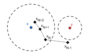
As discussed, we have already shown a sequence with a bounded finite range always has convergent subsequences. Now we prove the case where the range of the sequence of values $\left{a_{1}, a_{2} \ldots,\right$,$} has$ infinitely many distinct values. We assume the sequences start at $n=k$ and by assumption, there is a positive number $B$ so that $-B \leq a_{n} \leq B$ for all $n \geq k$. Define the interval $J_{0}=\left[\alpha_{0}, \beta_{0}\right]$ where $\alpha_{0}=-B$ and $\beta_{0}=B$. Thus at this starting step, $J_{0}=[-B, B]$. Note the length of $J_{0}$, denoted by $\ell_{0}$ is $2 B$.
Let $\mathcal{S}$ be the range of the sequence which has infinitely many points and for convenience, we will let the phrase infinitely many points be abbreviated to IMPs.
Step 1:
Bisect $\left[\alpha_{0}, \beta_{0}\right]$ into two pieces $u_{0}$ and $u_{1}$. That is the interval $J_{0}$ is the union of the two sets $u_{0}$ and $u_{1}$ and $J_{0}=u_{0} \cup u_{1}$. Now at least one of the intervals $u_{0}$ and $u_{1}$ contains IMPs of $\mathcal{S}$ as otherwise each piece has only finitely many points and that contradicts our assumption that $\mathcal{S}$ has IMPS. Now both may contain IMPS so select one such interval containing IMPS and call it $J_{1}$. Label the endpoints of $J_{1}$ as $\alpha_{1}$ and $\beta_{1}$; hence, $J_{1}=\left[\alpha_{1}, \beta_{1}\right] .$ Note $\ell_{1}=\beta_{1}-\alpha_{1}=\frac{1}{2} \ell_{0}=B$ We see $J_{1} \subseteq J_{0}$ and
$$
-B=\alpha_{0} \leq \alpha_{1} \leq \beta_{1} \leq \beta_{0}=B
$$
Since $J_{1}$ contains IMPS, we can select a sequence value $a_{n_{1}}$ from $J_{1}$.
Step 2:
Now bisect $J_{1}$ into subintervals $u_{0}$ and $u_{1}$ just as before so that $J_{1}=u_{0} \cup u_{1}$. At least one of $u_{0}$ and $u_{1}$ contain IMPS of $\mathcal{S}$.
Choose one such interval and call it $J_{2}$. Label the endpoints of $J_{2}$ as $\alpha_{2}$ and $\beta_{2}$; hence, $J_{2}=$ $\left[\alpha_{2}, \beta_{2}\right]$. Note $\ell_{2}=\beta_{2}-\alpha_{2}=\frac{1}{2} \ell_{1}$ or $\ell_{2}=(1 / 4) \ell_{0}=\left(1 / 2^{2}\right) \ell_{0}=(1 / 2) B$. We see $J_{2} \subseteq J_{1} \subseteq J_{0}$ and
$$
-B=\alpha_{0} \leq \alpha_{1} \leq \alpha_{2} \leq \beta_{2} \leq \beta_{1} \leq \beta_{0}=B
$$
数学代写|实变函数作业代写Real analysis代考|Extensions to $\Re^{2}$
We can extend our arguments to bounded sequences in $\mathfrak{R}^{2}$. We haven’t talked about it yet, but given a sequence in $\Re^{2}$, the elements of the sequence will be vectors. The sequence then will be made up of vectors.
$$
\left(\left(x_{n}\right)\right)=\left[\begin{array}{l}
x_{1, n} \
x_{2, n}
\end{array}\right]
$$
We would say the sequence converges to a vector $\boldsymbol{x}$ is for all $\epsilon>0$, there is an $N$ so that
$$
n>N \Longrightarrow\left|\boldsymbol{x}{n}-\boldsymbol{x}\right|{2}<\epsilon
$$
where we measure the distance between two vectors in $\Re^{2}$ using the standard Euclidean norm, here called $|\cdot|_{2}$ defined by
$$
\left|\boldsymbol{x}{n}-\boldsymbol{x}\right|{2}=\sqrt{\left(x_{1, n}-x_{1}\right)^{2}+\left(x_{2, n}-x_{2}\right)^{2}}
$$
where $\boldsymbol{x}=\left[x_{1}, x_{2}\right]^{\prime}$. This sequence is bounded if there is a positive number $B$ so that $\left|\boldsymbol{x}{\boldsymbol{n}}\right|{2}<B$ for all appropriate $n$. We can sketch the proof for the case where there are infinitely many vectors in this sequence which is bounded.
Theorem 4.2.2 The Bolzano – Weierstrass Theorem in $\Re^{2}$
Every bounded sequence of vectors in $\mathrm{R}^{2}$ with an infinite range has at least one convergent subsequence.
Proof 4.2.3
We will just sketch the argument. Since this sequence is bounded, there are positive numbers $B_{1}$ and $B_{2}$ so that
$$
-B_{1} \leq x_{1 n} \leq B_{1} \quad \text { and } \quad-B_{2} \leq x_{2 n} \leq B_{2}
$$
The same argument we just used for the Bolzano – Weierstrass Theorem in $\Re$ works. We bisect both edges of the box to create 4 rectangles. At least one must contain IMPs and we choose one that does. Then at each step, continue this subdivision process always choosing a rectangle with IMPs. Here are a few of the details. We start by labeling the initial box by
$$
J_{0}=\left[-B_{1}, B_{1}\right] \times\left[-B_{2}, B_{2}\right]=\left[\alpha_{0}, \beta_{0}\right] \times\left[\delta_{0}, \gamma 0\right]
$$
We pick a first vector $x_{n_{0}}$ from the initial box. The area of this rectangle is $A_{0}=\left(\beta_{0}-\alpha_{0}\right)\left(\gamma_{0}-\delta_{0}\right)$ and at the first step, the bisection of each edge leads to four rectangles of area $A_{0} / 4$. At least one of these rectangles contains IMPs and after our choice, we label the new rectangle. $J_{1}=\left[\alpha_{1}, \beta_{1}\right] \times$ $\left[\delta_{1}, \gamma_{1}\right]$ and pick a vector $\boldsymbol{x}{n{1}}$ different from the first one from $J_{0}$.
At this point, we have
$$
\begin{aligned}
&-B_{1}=\alpha_{0} \leq \alpha_{1} \leq \beta_{1} \leq \beta_{0}=B_{1} \
&-B_{2}=\delta_{0} \leq \delta_{1} \leq \gamma_{1} \leq \gamma_{0}=B_{2}
\end{aligned}
$$
and after $p$ steps, we have
$$
\begin{aligned}
&-B_{1}=\alpha_{0} \leq \alpha_{1} \leq \ldots \alpha_{p} \leq \beta_{p} \leq \ldots \leq \beta_{1} \leq \beta_{0}=B_{1} \
&-B_{2}=\delta_{0} \leq \delta_{1} \leq \ldots \delta_{p} \leq \gamma_{p} \leq \ldots \leq \gamma_{1} \leq \gamma_{0}=B_{2}
\end{aligned}
$$
with the edge lengths $\beta_{p}-\alpha_{p}$ and $\gamma_{p}-\delta_{p}$ going to zero as $p$ increases, As before, we pick a value $\boldsymbol{x}{n{p}}$ different from the ones at previous stages. Similar arguments show that $\alpha_{p} \rightarrow \alpha$ and $\beta_{p} \rightarrow \beta$ with $\alpha=\beta$ and $\delta_{p} \rightarrow \delta$ and $\gamma_{p} \rightarrow \gamma$ with $\delta=\gamma$. We find also $\boldsymbol{x}{n{p}} \rightarrow[\alpha, \delta]^{\prime}$ which gives us the result. The convergence arguments here are indeed a bit different as we have to measure distance between two vectors using $\left|_{1}\right|_{2}$ but it is not too difficult to figure it out.
实变函数代写
数学代写|实变函数作业代写Real analysis代考|Bounded Sequences with a Finite Range
我们已经看过有限范围的序列。由于它们的范围是有限的,因此它们是有界序列。我们也知道它们有我们已经明确计算过的收敛子序列。如果序列的范围是单个值,那么我们知道序列将收敛到该值,并且我们现在知道如何证明序列的收敛性。让我们将其形式化为一个定理。但这一次,我们将更抽象地争论。请注意论点如何仍然基本相同。
定理 4.1.1 具有有限范围的序列发散,除非范围是一个值
让序列(一种n)有一个有限的范围\left{y_{1}, \ldots, y_{p}\right}\left{y_{1}, \ldots, y_{p}\right}对于一些正整数p≥1. 如果p=1, 序列收敛到是1而如果p>1,序列不收敛但有子序列(一种nķ一世)收敛到是一世对于每个是一世在序列范围内。
证明 4.1.1
如果序列的范围只包含一个点,那么一种n=是1对全部n很容易看出一种n→是1如给定的ε>0,|一种n−是1|=|是1−是1|=0<ε对全部n这表明收敛。
如果范围有p>1, 让 a 为不在范围内的任何数字并计算d一世=|一种−是一世|, a 到每个点的距离是一世在范围内。让d=(1 / 2) \min \left{d_{1}, \ldots, d_{p}\right}d=(1 / 2) \min \left{d_{1}, \ldots, d_{p}\right}并选择ε=d. 然后|一种n−一种|承担p价值观,|是一世−一种|=d一世对全部n. 但d一世>d对全部一世这向我们展示了|一种n−一种|>ε对全部n. 稍加思考,我们就知道这正是序列的定义(一种n)不收敛到一种.
如果一种是范围值之一,比如说一种=是一世,那么我们上面定义的距离是正的,除了d一世这是零。所以|一种n−是一世|所有指数为零n给出范围值是一世但对所有其他范围值都是正数。让ε=d=(1/2)分钟j≠一世|d一世−dj|. 然后,对于任何索引n和一种n≠是一世, 我们有|一种n−是一世|=|是j−是一世|=dj>d对于一些j. 因此,无论怎样ñ我们挑选,我们总能找到n>ñ给予|一种n−是一世|>ε. 因此,极限不能是一世. 由于此参数适用于任何范围值是一世,我们看到限制值不能是任何范围值。
为了具体说明,假设范围内有 3 个值,\left{y_{1}, y_{2}, y_{3}\right}\left{y_{1}, y_{2}, y_{3}\right}. 如果限制是是2, 让\epsilon=d=(1 / 2) \min \left{\left|y_{1}-y_{2}\right|,\left|y_{3}-y_{2}\right|\right}\epsilon=d=(1 / 2) \min \left{\left|y_{1}-y_{2}\right|,\left|y_{3}-y_{2}\right|\right}. 然后,
|一种n−是2|={|是2−是1|>d=ε,一种n=是1 |是2−是2|=0,一种n=是2 |是3−是2|>d,=ε一种n=是3
鉴于任何ñ我们可以选择n>ñ以便|一种n−是2|>ε. 因此,极限不能是2. 请注意,这个论点比我们之前的论点要抽象得多。
注释 4.1.1 为了方便说明(很酷的短语……),让我们看一下范围值是1. 该序列有一个重复的块,在该块内是范围的不同值是一世. 有第一次是1存在于第一个块中。调用这个索引n1. 让块大小为问. 然后下次是1发生在块中的这个位置是在索引处n1+问. 实际上,是1出现在索引处的序列中n1+j问在哪里j≥1. 这定义了子序列一种n1+j问收敛到是1. 剩下的每一个都可以使用相同类型的参数是一世.
数学代写|实变函数作业代写Real analysis代考|Sequences with an Infinite Range
我们现在已经为我们迄今为止最抽象的结果做好了准备。
定理 4.2.1 Bolzano – Weierstrass Theorem
每个有界序列至少有一个收敛子序列。
证明 4.2.1
正如所讨论的,我们已经证明了一个有界有限范围的序列总是有收敛的子序列。现在我们证明值序列的范围\left{a_{1}, a_{2} \ldots,\right$,$} 有\left{a_{1}, a_{2} \ldots,\right$,$} 有无限多个不同的值。我们假设序列开始于n=ķ并且通过假设,有一个正数乙以便−乙≤一种n≤乙对全部n≥ķ. 定义间隔Ĵ0=[一种0,b0]在哪里一种0=−乙和b0=乙. 因此,在这个起始步骤,Ĵ0=[−乙,乙]. 注意长度Ĵ0,表示为ℓ0是2乙.
让小号是具有无限多点的序列的范围,为方便起见,我们将把无限多点这一短语缩写为 IMPs。
第 1 步:
平分[一种0,b0]分成两块在0和在1. 那就是间隔Ĵ0是两个集合的并集在0和在1和Ĵ0=在0∪在1. 现在至少有一个区间在0和在1包含 IMP小号因为否则每一块只有有限多的点,这与我们的假设相矛盾小号有 IMPS。现在两者都可能包含 IMPS,因此选择一个包含 IMPS 的间隔并调用它Ĵ1. 标记端点Ĵ1作为一种1和b1; 因此,Ĵ1=[一种1,b1].笔记ℓ1=b1−一种1=12ℓ0=乙我们看Ĵ1⊆Ĵ0和
−乙=一种0≤一种1≤b1≤b0=乙
自从Ĵ1包含 IMPS,我们可以选择一个序列值一种n1从Ĵ1.
第2步:
现在平分Ĵ1进入子区间在0和在1就像以前一样Ĵ1=在0∪在1. 至少其中之一在0和在1包含 IMPS小号.
选择一个这样的间隔并调用它Ĵ2. 标记端点Ĵ2作为一种2和b2; 因此,Ĵ2= [一种2,b2]. 笔记ℓ2=b2−一种2=12ℓ1或者ℓ2=(1/4)ℓ0=(1/22)ℓ0=(1/2)乙. 我们看Ĵ2⊆Ĵ1⊆Ĵ0和
−乙=一种0≤一种1≤一种2≤b2≤b1≤b0=乙
数学代写|实变函数作业代写Real analysis代考|Extensions to ℜ2
我们可以将我们的论点扩展到有界序列R2. 我们还没有谈论它,但给出了一个序列ℜ2,序列的元素将是向量。然后序列将由向量组成。
((Xn))=[X1,n X2,n]
我们会说序列收敛到一个向量X适合所有人ε>0, 有一个ñ以便
n>ñ⟹|Xn−X|2<ε
我们测量两个向量之间的距离ℜ2使用标准欧几里得范数,这里称为|⋅|2被定义为
|Xn−X|2=(X1,n−X1)2+(X2,n−X2)2
在哪里X=[X1,X2]′. 如果有一个正数,这个序列是有界的乙以便|Xn|2<乙对于所有适当的n. 我们可以勾勒出这个有界序列中有无限多个向量的情况的证明。
定理 4.2.2 Bolzano – Weierstrass Theorem inℜ2
中的每个有界向量序列R2具有无限范围的至少有一个收敛子序列。
证明 4.2.3
我们将简述论证。由于这个序列是有界的,所以有正数乙1和乙2以便
−乙1≤X1n≤乙1 和 −乙2≤X2n≤乙2
我们刚刚对 Bolzano – Weierstrass Theorem 使用的相同论点ℜ作品。我们将盒子的两条边一分为二来创建 4 个矩形。至少一个必须包含 IMP,我们选择一个包含 IMP。然后在每一步,继续这个细分过程,总是选择一个带有 IMP 的矩形。这里有一些细节。我们首先将初始框标记为
Ĵ0=[−乙1,乙1]×[−乙2,乙2]=[一种0,b0]×[d0,C0]
我们选择第一个向量Xn0从最初的盒子。这个矩形的面积是一种0=(b0−一种0)(C0−d0)第一步,每条边的二等分导致四个矩形区域一种0/4. 这些矩形中至少有一个包含 IMP,在我们选择之后,我们标记新的矩形。Ĵ1=[一种1,b1]× [d1,C1]并选择一个向量Xn1不同于第一个Ĵ0.
此时,我们有
−乙1=一种0≤一种1≤b1≤b0=乙1 −乙2=d0≤d1≤C1≤C0=乙2
之后p步骤,我们有
−乙1=一种0≤一种1≤…一种p≤bp≤…≤b1≤b0=乙1 −乙2=d0≤d1≤…dp≤Cp≤…≤C1≤C0=乙2
边长bp−一种p和Cp−dp归零为p增加,和以前一样,我们选择一个值Xnp与之前的阶段不同。类似的论据表明一种p→一种和bp→b和一种=b和dp→d和Cp→C和d=C. 我们还发现Xnp→[一种,d]′这给了我们结果。这里的收敛参数确实有点不同,因为我们必须使用测量两个向量之间的距离|1|2但弄清楚它并不难。

统计代写请认准statistics-lab™. statistics-lab™为您的留学生涯保驾护航。
金融工程代写
金融工程是使用数学技术来解决金融问题。金融工程使用计算机科学、统计学、经济学和应用数学领域的工具和知识来解决当前的金融问题,以及设计新的和创新的金融产品。
非参数统计代写
非参数统计指的是一种统计方法,其中不假设数据来自于由少数参数决定的规定模型;这种模型的例子包括正态分布模型和线性回归模型。
广义线性模型代考
广义线性模型(GLM)归属统计学领域,是一种应用灵活的线性回归模型。该模型允许因变量的偏差分布有除了正态分布之外的其它分布。
术语 广义线性模型(GLM)通常是指给定连续和/或分类预测因素的连续响应变量的常规线性回归模型。它包括多元线性回归,以及方差分析和方差分析(仅含固定效应)。
有限元方法代写
有限元方法(FEM)是一种流行的方法,用于数值解决工程和数学建模中出现的微分方程。典型的问题领域包括结构分析、传热、流体流动、质量运输和电磁势等传统领域。
有限元是一种通用的数值方法,用于解决两个或三个空间变量的偏微分方程(即一些边界值问题)。为了解决一个问题,有限元将一个大系统细分为更小、更简单的部分,称为有限元。这是通过在空间维度上的特定空间离散化来实现的,它是通过构建对象的网格来实现的:用于求解的数值域,它有有限数量的点。边界值问题的有限元方法表述最终导致一个代数方程组。该方法在域上对未知函数进行逼近。[1] 然后将模拟这些有限元的简单方程组合成一个更大的方程系统,以模拟整个问题。然后,有限元通过变化微积分使相关的误差函数最小化来逼近一个解决方案。
tatistics-lab作为专业的留学生服务机构,多年来已为美国、英国、加拿大、澳洲等留学热门地的学生提供专业的学术服务,包括但不限于Essay代写,Assignment代写,Dissertation代写,Report代写,小组作业代写,Proposal代写,Paper代写,Presentation代写,计算机作业代写,论文修改和润色,网课代做,exam代考等等。写作范围涵盖高中,本科,研究生等海外留学全阶段,辐射金融,经济学,会计学,审计学,管理学等全球99%专业科目。写作团队既有专业英语母语作者,也有海外名校硕博留学生,每位写作老师都拥有过硬的语言能力,专业的学科背景和学术写作经验。我们承诺100%原创,100%专业,100%准时,100%满意。
随机分析代写
随机微积分是数学的一个分支,对随机过程进行操作。它允许为随机过程的积分定义一个关于随机过程的一致的积分理论。这个领域是由日本数学家伊藤清在第二次世界大战期间创建并开始的。
时间序列分析代写
随机过程,是依赖于参数的一组随机变量的全体,参数通常是时间。 随机变量是随机现象的数量表现,其时间序列是一组按照时间发生先后顺序进行排列的数据点序列。通常一组时间序列的时间间隔为一恒定值(如1秒,5分钟,12小时,7天,1年),因此时间序列可以作为离散时间数据进行分析处理。研究时间序列数据的意义在于现实中,往往需要研究某个事物其随时间发展变化的规律。这就需要通过研究该事物过去发展的历史记录,以得到其自身发展的规律。
回归分析代写
多元回归分析渐进(Multiple Regression Analysis Asymptotics)属于计量经济学领域,主要是一种数学上的统计分析方法,可以分析复杂情况下各影响因素的数学关系,在自然科学、社会和经济学等多个领域内应用广泛。
MATLAB代写
MATLAB 是一种用于技术计算的高性能语言。它将计算、可视化和编程集成在一个易于使用的环境中,其中问题和解决方案以熟悉的数学符号表示。典型用途包括:数学和计算算法开发建模、仿真和原型制作数据分析、探索和可视化科学和工程图形应用程序开发,包括图形用户界面构建MATLAB 是一个交互式系统,其基本数据元素是一个不需要维度的数组。这使您可以解决许多技术计算问题,尤其是那些具有矩阵和向量公式的问题,而只需用 C 或 Fortran 等标量非交互式语言编写程序所需的时间的一小部分。MATLAB 名称代表矩阵实验室。MATLAB 最初的编写目的是提供对由 LINPACK 和 EISPACK 项目开发的矩阵软件的轻松访问,这两个项目共同代表了矩阵计算软件的最新技术。MATLAB 经过多年的发展,得到了许多用户的投入。在大学环境中,它是数学、工程和科学入门和高级课程的标准教学工具。在工业领域,MATLAB 是高效研究、开发和分析的首选工具。MATLAB 具有一系列称为工具箱的特定于应用程序的解决方案。对于大多数 MATLAB 用户来说非常重要,工具箱允许您学习和应用专业技术。工具箱是 MATLAB 函数(M 文件)的综合集合,可扩展 MATLAB 环境以解决特定类别的问题。可用工具箱的领域包括信号处理、控制系统、神经网络、模糊逻辑、小波、仿真等。