如果你也在 怎样代写数论number theory这个学科遇到相关的难题,请随时右上角联系我们的24/7代写客服。
数论是纯数学的一个分支,主要致力于研究整数和整数值函数。数论是对正整数集合的研究。
statistics-lab™ 为您的留学生涯保驾护航 在代写数论number theory方面已经树立了自己的口碑, 保证靠谱, 高质且原创的统计Statistics代写服务。我们的专家在代写数论number theory代写方面经验极为丰富,各种代写数论number theory相关的作业也就用不着说。
我们提供的数论number theory及其相关学科的代写,服务范围广, 其中包括但不限于:
- Statistical Inference 统计推断
- Statistical Computing 统计计算
- Advanced Probability Theory 高等概率论
- Advanced Mathematical Statistics 高等数理统计学
- (Generalized) Linear Models 广义线性模型
- Statistical Machine Learning 统计机器学习
- Longitudinal Data Analysis 纵向数据分析
- Foundations of Data Science 数据科学基础
数学代写|数论作业代写number theory代考|Courant’s Nodal Domain Theorem
Let $\phi$ be an eigenfunction of (1.1). The nodal set $\mathcal{Z}(\phi)$ of $\phi$ is defined as the closure of the set of (interior) zeros of $\phi$,
$$
\mathcal{Z}(\phi):=\overline{{x \in \Omega \mid \phi(x)=0}}
$$
A nodal domain of $\phi$ is a connectèd component of the set $\Omega \backslash \mathcal{Z}(\phi)$. Cäll $\beta_{0}(\phi)$ the number of nodal domains of $\phi$. We recall the following classical theorem $[12$, Chap. VI.6].
Theorem 1.1 (Courant 1923) Assume that the eigenvalues of (1.1) are listed in non-decreasing order, with multiplicities,
$$
\mu_{1}<\mu_{2} \leq \mu_{3} \leq \cdots
$$
Then, for any eigenfunction $\phi \in \mathcal{E}(\mu)$ of $(1.1)$, associated with the eigenvalue $\mu$,
$$
\beta_{0}(\phi) \leq \kappa(\mu)
$$
In particular, any $\phi \in \mathcal{E}\left(\mu_{k}\right)$ has a most $k$ nodal domains,
Courant’s theorem is a partial generalization, to higher dimensions, of a classical theorem of C. Sturm (1836). Indeed, in dimension 1, a $k$ th eigenfunction of the Sturm-Liouville operator $-\frac{d^{2}}{d x^{2}}+q(x)$ in $] a, b[$, with Dirichlet, Neumann, or mixed Dirichlet-Neumann boundary condition at ${a, b}$, has exactly $k$ nodal domains in ]$a, b[$. In dimension 2 (or higher), Courant’s theorem is not sharp. On the one hand, Stern (1925) proved that for the square with Dirichlet boundary condition, or for the 2-sphere, there exist eigenfunctions of arbitrarily high energy, with exactly two or
three nodal domains. On the other hand, Pleijel (1956) proved that, for any bounded domain in $\mathbb{R}^{2}$, there are only finitely many Dirichlet eigenvalues for which Courant’s theorem is sharp. We refer to $[7,24]$ for more details, and to [20] for Pleijel’s estimate under Neumann boundary condition.
Another remarkable theorem of Sturm states that any non trivial linear combination $u=\sum_{k=m}^{n} a_{j} u_{j}$ of eigenfunctions of the operator $-\frac{d^{2}}{d x^{2}}+q(x)$ has at most $(n-1)$ zeros (counted with multiplicities), and at least $(m-1)$ sign changes in the interval $] a, b[$, see [10].
A footnote in [12, p. 454], states that Courant’s theorem may be generalized as follows: Any linear combination of the first $n$ eigenfunctions divides the domain, by means of its nodes, into no more than $n$ subdomains. See the Göttingen dissertation of H. Herrmann, Beiträge zur Theorie der Eigenwerten und Eigenfunktionen, $1932 .$ For later reference, we introduce the following definition.
数学代写|数论作业代写number theory代考|Symmetries and Spectra
In this subsection, we analyze how symmetries influence the structure of the eigenvalues and eigenfunctions. The analysis is carried out for the equilateral rhombus, but the basic ideas work for the regular hexagon as well, and will be used in Sect. 3 .
In the sequel, we denote by the same letter $L$ a line in $\mathbb{R}^{2}$, and the mirror symmetry with respect to this line. We denote by $L^{}$ the action of the symmetry $L$ on functions, $L^{} \phi=\phi \circ L$.
A function $\phi$ is even (or invariant) with respect to $L$ if $L^{} \phi=\phi$. It is odd (or anti-invariant) with respect to $L$ if $L^{} \phi=-\phi$. In the former case, the line $L$ is an anti-nodal line for $\phi$, i.e., the normal derivative $v_{L} \cdot \phi$ is zero along $L$, where $v_{L}$ denotes a unit field normal to $L$ along $L$. In the latter case, the line $L$ is a nodal line for $\phi$, i.e., $\phi$ vanishes along $L$.
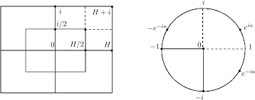
Let $\mathcal{R} h_{e}$ be the interior of the equilateral rhombus with sides of length 1 , and verticês $\left.\left(-\frac{\sqrt{3}}{2}, 0\right),\left(0,-\frac{1}{2}\right),\left(\frac{\sqrt{3}}{2}\right), 0\right)$ ând $\left(0, \frac{1}{2}\right)$. Câll $D$ ând $M$ its diagononâls (rêsp̄. the longer one and the shorter one). The diagonal $M$ divides the rhombus into two equilateral triangles. The diagonals $D$ and $M$ divide the rhombus into four hemiequilateral triangles. In the sequel, we use the generic notation $\mathcal{T}{e}$ (resp. $\mathcal{T}{h}$ ) for any of the equilateral triangles (resp. hemiequilateral triangles) into which the rhombus decomposes, see Fig. 1 .
For $L \in{D, M}$, define the sets
$$
\left{\begin{array}{l}
\mathcal{S}{L,+}=\left{\phi \in L^{2}\left(\mathcal{R} h{e}\right) \mid L^{} \phi=+\phi\right. \ \mathcal{S}{L,-}=\left{\phi \in L^{2}\left(\mathcal{R} h{e}\right) \mid L^{} \phi=-\phi\right.
\end{array}\right}
$$
数学代写|数论作业代写number theory代考|Riemann-Schwarz Reflection Principle
In this subsection, we recall the “Riemann-Schwarz reflection principle” which we will use repeatedly in the sequel.
Consider the decomposition $\mathcal{R} h_{e}=\mathcal{T}{e, 1} \bigsqcup \mathcal{T}{e, 2}$, with $M\left(\mathcal{T}{e, 1}\right)=\mathcal{T}{e, 2}$. Choose a boundary condition $\mathfrak{a} \in{\mathfrak{d}, \mathrm{n}}$ on $\partial \mathcal{R} h_{e}$. Given an eigenvalue $\lambda$ of $-\Delta$ for $\left(\mathcal{R} h_{e}, \mathfrak{a}\right)$,
and $\sigma \in{+,-}$, consider the subspace $\mathcal{E}(\lambda) \cap \mathcal{S}{M, \sigma}$ of eigenfunctions $\phi \in \mathcal{E}(\lambda)$ such that $M^{} \phi=\sigma \phi$. If $0 \neq \phi \in \mathcal{E}(\lambda) \cap \mathcal{S}{M, \sigma}$, then $\phi \mid \mathcal{T}{e, 1}$ is an eigenfunction of $-\Delta$ for $\left(\mathcal{T}{e, 1}, \mathfrak{a} \mathfrak{b}\right)$,
with $\mathfrak{b}=\mathfrak{n}$ if $\sigma=+$, and $\mathfrak{b}=\mathfrak{d}$ if $\sigma=-$, associated with the same eigenvalue $\lambda$.
Conversely, let $\psi$ be an eigenfunction of $\left(\mathcal{T}{e, 1}, \mathfrak{a} \mathfrak{a} \mathfrak{b}\right)$, with eigenvalue $\mu{m}\left(\mathcal{T}{e, 1}, \mathfrak{a} \mathfrak{a} \mathfrak{b}\right)$, for some $m \geq 1$. Define the function $\breve{\psi}$ on $\mathcal{R} h{e}$ such that $\breve{\psi} \mid \mathcal{T}{e, 1}=\psi$ and $\breve{\psi} \mid \mathcal{T}{e, 2}=$
and $\sigma \in{+,-}$, consider the subspace $\mathcal{E}(\lambda) \cap \mathcal{S}{M, \sigma}$ of eigenfunctions $\phi \in \mathcal{E}(\lambda)$ such that $M^{} \phi=\sigma \phi$.
If $0 \neq \phi \in \mathcal{E}(\lambda) \cap \mathcal{S}{M, \sigma}$, then $\phi \mid \mathcal{T}{e, 1}$ is an eigenfunction of $-\Delta$ for $\left(\mathcal{T}{e, 1}, \mathfrak{a a b}\right)$,
with $\mathfrak{b}=\mathfrak{n}$ if $\sigma=+$, and $\mathfrak{b}=\mathfrak{d}$ if $\sigma=-$, associated with the same eigenvalue $\lambda$.
Conversely, let $\psi$ be an eigenfunction of $\left(\mathcal{T}{e, 1}, \mathfrak{a} \mathfrak{a} b\right)$, with eigenvalue $\mu{m}\left(\mathcal{T}{e, 1}\right.$, a a $\left.\mathfrak{b}\right)$, for some $m \geq 1$. Define the function $\breve{\psi}$ on $\mathcal{R} h{e}$ such that $\breve{\psi} \mid \mathcal{T}{e, 1}=\psi$ and $\breve{\psi} \mid \mathcal{T}{e, 2}=$
$\sigma \psi \circ M$. This means that $\breve{\psi}$ is obtained by extending $\psi$ across $M$ to $\mathcal{T}{e, 2}$ by sym- metry, in such a way that $M^{} \breve{\psi}=\sigma \breve{\psi}$. It is easy to see that the function $\bar{\psi}$ is an eigenfunction of $-\Delta$ for $\left(\mathcal{R} h{e}, \mathfrak{a}\right)$ (in particular it is smooth in a neighborhood of
$M)$, with eigenvalue $\mu_{m}\left(\mathcal{T}{e, 1}, \mathfrak{a a b}\right)$, so that $\breve{\psi} \in \mathcal{E}\left(\mu{m}\right) \cap \mathcal{S}{M, \sigma}$. The above considerations prove the first two assertions in the following proposi- tion. The proof of the third and fourth assertions is similar, using the symmetries $D$ and $M$, and the decomposition of $\mathcal{R} h{e}$ into hemiequilateral triangles $\mathcal{T}{h, j}, 1 \leq j \leq 4$. $\sigma \psi \circ M$. This means that $\psi$ is obtained by extending $\psi$ across $M$ to $\mathcal{T}{e, 2}$ by sym-
metry, in such a way that $M^{} \psi=\sigma \breve{\psi}$. It is easy to see that the function $\dot{\psi}$ is an
eigenfunction of $-\Delta$ for $\left(\mathcal{R} h_{e}\right.$, a) (in particular it is smooth in a neighborhood of
$M)$, with eigenvalue $\mu_{m}\left(\mathcal{T}{e, 1}, \mathfrak{a} a \mathfrak{b}\right)$, so that $\breve{\psi} \in \mathcal{E}\left(\mu{m}\right) \cap \mathcal{S}{M, \sigma}$. The above considerations prove the first two assertions in the following proposition. The proof of the third and fourth assertions is similar, using the symmetries $D$ and $M$, and the decomposition of $\mathcal{R} h{e}$ into hemiequilateral triangles $\mathcal{T}_{h, j}, 1 \leq j \leq 4$.
数论作业代写
数学代写|数论作业代写number theory代考|Courant’s Nodal Domain Theorem
让φ是 (1.1) 的特征函数。节点集从(φ)的φ被定义为(内部)零点集合的闭包φ,
从(φ):=X∈Ω∣φ(X)=0¯
一个节点域φ是集合的连通分量Ω∖从(φ). 称呼b0(φ)的节点域数φ. 我们回顾以下经典定理[12,章。六.6]。
定理 1.1 (Courant 1923) 假设 (1.1) 的特征值按非递减顺序列出,具有多重性,
μ1<μ2≤μ3≤⋯
那么,对于任何特征函数φ∈和(μ)的(1.1),与特征值相关联μ,
b0(φ)≤ķ(μ)
特别是,任何φ∈和(μķ)有一个最ķ节点域,
Courant 定理是 C. Sturm (1836) 的经典定理向更高维度的部分推广。实际上,在维度 1 中,aķSturm-Liouville 算子的特征函数−d2dX2+q(X)在]一个,b[, Dirichlet、Neumann 或混合 Dirichlet-Neumann 边界条件为一个,b, 正好ķ]中的节点域一个,b[. 在维度 2(或更高维度)中,Courant 定理并不尖锐。一方面,Stern (1925) 证明,对于具有 Dirichlet 边界条件的正方形,或者对于 2 球体,存在任意高能量的特征函数,恰好有两个或
三个节点域。另一方面,Pleijel (1956) 证明,对于任何有界域R2,只有有限多个 Dirichlet 特征值,Courant 的定理是尖锐的。我们指[7,24]有关更多详细信息,请参阅 [20] 在 Neumann 边界条件下的 Pleijel 估计。
Sturm 的另一个显着定理指出,任何非平凡的线性组合在=∑ķ=米n一个j在j算子的特征函数−d2dX2+q(X)最多有(n−1)零(以重数计算),并且至少(米−1)区间内的符号变化]一个,b[,见[10]。
[12, p. 中的脚注。454],指出 Courant 定理可以概括如下:neigenfunctions 通过其节点将域划分为不超过n子域。参见 H. Herrmann 的 Göttingen 论文,Contributions to the theory of eigenvalues and eigenfunctions,1932.为了以后的参考,我们引入以下定义。
数学代写|数论作业代写number theory代考|Symmetries and Spectra
在本小节中,我们将分析对称性如何影响特征值和特征函数的结构。分析是针对等边菱形进行的,但基本思想也适用于正六边形,将在 Sect. 3.
在续集中,我们用相同的字母表示大号一条线R2,以及关于这条线的镜像对称。我们表示大号对称的作用大号关于功能,大号φ=φ∘大号.
一个函数φ是偶数(或不变)关于大号如果大号φ=φ. 它是奇数的(或反不变的)关于大号如果大号φ=−φ. 在前一种情况下,行大号是一条反节点线φ,即正常导数在大号⋅φ沿为零大号, 在哪里在大号表示一个单位域,垂直于大号沿着大号. 在后一种情况下,行大号是一条节点线φ, IE,φ随之消失大号.
让RH和是边长为 1 和顶点的等边菱形的内部(−32,0),(0,−12),(32),0)母鸡(0,12). 凝乳D母鸡米它的对角线(rêsp̄。较长的和较短的)。对角线米将菱形分成两个等边三角形。对角线D和米将菱形分成四个半等边三角形。在续集中,我们使用通用符号吨和(分别。吨H) 对于菱形分解成的任何等边三角形(分别是半等边三角形),参见图 1。
为了大号∈D,米, 定义集合
$$
\left{\begin{array}{l}
\mathcal{S}{L,+}=\left{\phi \in L^{2}\left(\mathcal{R} h{ e}\right) \mid L^{} \phi=+\phi\right. \ \mathcal{S}{L,-}=\left{\phi \in L^{2}\left(\mathcal{R} h{e}\right) \mid L^{} \phi=-\ φ\对。
\end{数组}\right}
$$
数学代写|数论作业代写number theory代考|Riemann-Schwarz Reflection Principle
在本小节中,我们回顾一下我们将在续集中重复使用的“黎曼-施瓦茨反射原理”。
考虑分解RH和=吨和,1⨆吨和,2, 和米(吨和,1)=吨和,2. 选择边界条件一个∈d,n在∂RH和. 给定一个特征值λ的−Δ为了(RH和,一个),
和σ∈+,−, 考虑子空间和(λ)∩小号米,σ特征函数φ∈和(λ)这样米φ=σφ. 如果0≠φ∈和(λ)∩小号米,σ, 然后φ∣吨和,1是一个特征函数−Δ为了(吨和,1,一个b),
与b=n如果σ=+, 和b=d如果σ=−,与相同的特征值相关联λ.
反之,让ψ是一个特征函数(吨和,1,一个一个b), 有特征值μ米(吨和,1,一个一个b), 对于一些米≥1. 定义函数ψ˘在RH和这样ψ˘∣吨和,1=ψ和ψ˘∣吨和,2=
和σ∈+,−, 考虑子空间和(λ)∩小号米,σ特征函数φ∈和(λ)这样米φ=σφ.
如果0≠φ∈和(λ)∩小号米,σ, 然后φ∣吨和,1是一个特征函数−Δ为了(吨和,1,一个一个b),
与b=n如果σ=+, 和b=d如果σ=−,与相同的特征值相关联λ.
反之,让ψ是一个特征函数(吨和,1,一个一个b), 有特征值μ米(吨和,1, 一个b), 对于一些米≥1. 定义函数ψ˘在RH和这样ψ˘∣吨和,1=ψ和ψ˘∣吨和,2=
σψ∘米. 这意味着ψ˘通过扩展获得ψ穿过米至吨和,2通过对称,以这样的方式米ψ˘=σψ˘. 很容易看出函数ψ¯是一个特征函数−Δ为了(RH和,一个)(特别是在附近很光滑
米), 有特征值μ米(吨和,1,一个一个b), 以便ψ˘∈和(μ米)∩小号米,σ. 上述考虑证明了以下命题中的前两个断言。第三个和第四个断言的证明是相似的,使用对称性D和米, 和分解RH和变成半等边三角形吨H,j,1≤j≤4. σψ∘米. 这意味着ψ通过扩展获得ψ穿过米至吨和,2通过对称
,以这样的方式米ψ=σψ˘. 很容易看出函数ψ˙是一个
特征函数−Δ为了(RH和, a) (特别是在
米), 有特征值μ米(吨和,1,一个一个b), 以便ψ˘∈和(μ米)∩小号米,σ. 上述考虑证明了以下命题中的前两个断言。第三个和第四个断言的证明是相似的,使用对称性D和米, 和分解RH和变成半等边三角形吨H,j,1≤j≤4.

统计代写请认准statistics-lab™. statistics-lab™为您的留学生涯保驾护航。
金融工程代写
金融工程是使用数学技术来解决金融问题。金融工程使用计算机科学、统计学、经济学和应用数学领域的工具和知识来解决当前的金融问题,以及设计新的和创新的金融产品。
非参数统计代写
非参数统计指的是一种统计方法,其中不假设数据来自于由少数参数决定的规定模型;这种模型的例子包括正态分布模型和线性回归模型。
广义线性模型代考
广义线性模型(GLM)归属统计学领域,是一种应用灵活的线性回归模型。该模型允许因变量的偏差分布有除了正态分布之外的其它分布。
术语 广义线性模型(GLM)通常是指给定连续和/或分类预测因素的连续响应变量的常规线性回归模型。它包括多元线性回归,以及方差分析和方差分析(仅含固定效应)。
有限元方法代写
有限元方法(FEM)是一种流行的方法,用于数值解决工程和数学建模中出现的微分方程。典型的问题领域包括结构分析、传热、流体流动、质量运输和电磁势等传统领域。
有限元是一种通用的数值方法,用于解决两个或三个空间变量的偏微分方程(即一些边界值问题)。为了解决一个问题,有限元将一个大系统细分为更小、更简单的部分,称为有限元。这是通过在空间维度上的特定空间离散化来实现的,它是通过构建对象的网格来实现的:用于求解的数值域,它有有限数量的点。边界值问题的有限元方法表述最终导致一个代数方程组。该方法在域上对未知函数进行逼近。[1] 然后将模拟这些有限元的简单方程组合成一个更大的方程系统,以模拟整个问题。然后,有限元通过变化微积分使相关的误差函数最小化来逼近一个解决方案。
tatistics-lab作为专业的留学生服务机构,多年来已为美国、英国、加拿大、澳洲等留学热门地的学生提供专业的学术服务,包括但不限于Essay代写,Assignment代写,Dissertation代写,Report代写,小组作业代写,Proposal代写,Paper代写,Presentation代写,计算机作业代写,论文修改和润色,网课代做,exam代考等等。写作范围涵盖高中,本科,研究生等海外留学全阶段,辐射金融,经济学,会计学,审计学,管理学等全球99%专业科目。写作团队既有专业英语母语作者,也有海外名校硕博留学生,每位写作老师都拥有过硬的语言能力,专业的学科背景和学术写作经验。我们承诺100%原创,100%专业,100%准时,100%满意。
随机分析代写
随机微积分是数学的一个分支,对随机过程进行操作。它允许为随机过程的积分定义一个关于随机过程的一致的积分理论。这个领域是由日本数学家伊藤清在第二次世界大战期间创建并开始的。
时间序列分析代写
随机过程,是依赖于参数的一组随机变量的全体,参数通常是时间。 随机变量是随机现象的数量表现,其时间序列是一组按照时间发生先后顺序进行排列的数据点序列。通常一组时间序列的时间间隔为一恒定值(如1秒,5分钟,12小时,7天,1年),因此时间序列可以作为离散时间数据进行分析处理。研究时间序列数据的意义在于现实中,往往需要研究某个事物其随时间发展变化的规律。这就需要通过研究该事物过去发展的历史记录,以得到其自身发展的规律。
回归分析代写
多元回归分析渐进(Multiple Regression Analysis Asymptotics)属于计量经济学领域,主要是一种数学上的统计分析方法,可以分析复杂情况下各影响因素的数学关系,在自然科学、社会和经济学等多个领域内应用广泛。
MATLAB代写
MATLAB 是一种用于技术计算的高性能语言。它将计算、可视化和编程集成在一个易于使用的环境中,其中问题和解决方案以熟悉的数学符号表示。典型用途包括:数学和计算算法开发建模、仿真和原型制作数据分析、探索和可视化科学和工程图形应用程序开发,包括图形用户界面构建MATLAB 是一个交互式系统,其基本数据元素是一个不需要维度的数组。这使您可以解决许多技术计算问题,尤其是那些具有矩阵和向量公式的问题,而只需用 C 或 Fortran 等标量非交互式语言编写程序所需的时间的一小部分。MATLAB 名称代表矩阵实验室。MATLAB 最初的编写目的是提供对由 LINPACK 和 EISPACK 项目开发的矩阵软件的轻松访问,这两个项目共同代表了矩阵计算软件的最新技术。MATLAB 经过多年的发展,得到了许多用户的投入。在大学环境中,它是数学、工程和科学入门和高级课程的标准教学工具。在工业领域,MATLAB 是高效研究、开发和分析的首选工具。MATLAB 具有一系列称为工具箱的特定于应用程序的解决方案。对于大多数 MATLAB 用户来说非常重要,工具箱允许您学习和应用专业技术。工具箱是 MATLAB 函数(M 文件)的综合集合,可扩展 MATLAB 环境以解决特定类别的问题。可用工具箱的领域包括信号处理、控制系统、神经网络、模糊逻辑、小波、仿真等。