如果你也在 怎样代写matlab这个学科遇到相关的难题,请随时右上角联系我们的24/7代写客服。
MATLAB是一个编程和数值计算平台,被数百万工程师和科学家用来分析数据、开发算法和创建模型。
MATLAB主要用于数值运算,但利用为数众多的附加工具箱,它也适合不同领域的应用,例如控制系统设计与分析、影像处理、深度学习、信号处理与通讯、金融建模和分析等。另外还有配套软件包提供可视化开发环境,常用于系统模拟、动态嵌入式系统开发等方面。
statistics-lab™ 为您的留学生涯保驾护航 在代写matlab方面已经树立了自己的口碑, 保证靠谱, 高质且原创的统计Statistics代写服务。我们的专家在代写matlab代写方面经验极为丰富,各种代写matlab相关的作业也就用不着说。
我们提供的matlab及其相关学科的代写,服务范围广, 其中包括但不限于:
- Statistical Inference 统计推断
- Statistical Computing 统计计算
- Advanced Probability Theory 高等概率论
- Advanced Mathematical Statistics 高等数理统计学
- (Generalized) Linear Models 广义线性模型
- Statistical Machine Learning 统计机器学习
- Longitudinal Data Analysis 纵向数据分析
- Foundations of Data Science 数据科学基础
数学代写|matlab仿真代写simulation代做|Closed Contour Equations
This study aims at providing an algebraic method to compute the velocities of a closed kinematic chain $[3,18,71]$. The method of independent contour (loop) equations is very efficient and can be applied to planar and spatial mechanical systems.
Consider two rigid bodies $(j)$ and $(k)$ connected by a joint or kinematic pair at $A$. The following relation exists between the velocity $\mathbf{v}{A}$ of the point $A{j}$ and the velocity $\mathbf{v}{A{k}}$ of the point $A_{k}$
$$
\mathbf{v}{A{j}}=\mathbf{v}{A{k}}+\mathbf{v}{A{j k},}^{r}
$$
where $\mathbf{v}{A{j k}}^{r}=\mathbf{v}{A{j} A_{k}}^{r}=\mathbf{v}{A{j} A_{k}}$ is the velocity of $A_{j}$ as seen by an observer at $A_{k}$ attached to body $(k)$ or the relative velocity of $A_{j}$ with respect to $A_{k}$, allowed at the joint $A$. The accelerations of $A_{j}$ and $A_{k}$ are expressed as
$$
\mathbf{a}{A{j}}=\mathbf{a}{A{k}}+\mathbf{a}{A{j k}}^{r}+\mathbf{a}{A{j k}}^{c},
$$
where $\mathbf{a}{A{j k}}^{r}=\mathbf{a}{A{j} A_{k}}^{r}=\mathbf{a}{A{j} A_{k}}$ is the relative acceleration of $A_{j}$ with respect to $A_{k}$ and $\mathbf{a}{A{j k}}^{c}=\mathbf{a}{A{j} A_{k}}^{c_{k}}$ is the Coriolis acceleration given by
$$
\mathbf{a}{A{j k}}^{c}=2 \boldsymbol{\omega}{k} \times \mathbf{v}{A j k}^{r},
$$
where $\omega_{k}$ is the angular velocity of the body $(k)$. Equations (3.1) and (3.2) are useful even for coincident points belonging to two rigid bodies that may not be directly
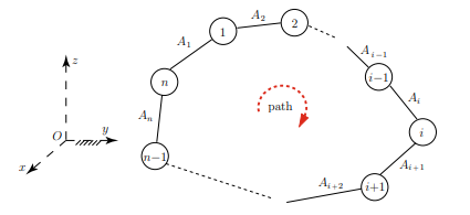
connected. Figure $3.1$ shows a monoloop closed kinematic chain with $n$ rigid links. The joint $A_{i}$ where $i=1,2, \ldots, n$ is the connection between the links $(i)$ and $(i-1)$. At the joint $A_{i}$ there are two instantaneously coincident points. The point $A_{i, i}$ belongs to link $(i), A_{i, i} \in(i)$ and the point $A_{i, i-1}$ belongs to body $(i-1), A_{i, i-1} \in(i-1)$. The absolute angular velocity of the rigid body ( $i$ ) is
$$
\omega_{i}=\omega_{i-1}+\omega_{i, i-1}
$$
where $\boldsymbol{\omega}{i, i-1}$ is the relative angular velocity of the rigid body (i) with respect to the rigid body $(i-1)$. For the $n$ link closed kinematic chain the equations for the angular velocities are $$ \boldsymbol{\omega}{1}=\boldsymbol{\omega}{n}+\boldsymbol{\omega}{1, n}: \boldsymbol{\omega}{2}=\boldsymbol{\omega}{1}+\boldsymbol{\omega}{2,1}: \ldots \boldsymbol{\omega}{i}=\boldsymbol{\omega}{i-1}+\boldsymbol{\omega}{i, i-1}: \ldots \boldsymbol{\omega}{n}=\boldsymbol{\omega}{n-1}+\boldsymbol{\omega}{n, n-1} \text { (3.5) } $$ Summing the expressions in Eq. (3.5) the following relation is obtained $$ \omega{1, n}+\omega_{2,1}+\ldots+\omega_{n, n-1}=\mathbf{0} \text { or } \sum_{(i)} \omega_{i, i-1}=\mathbf{0}
$$
The first vectorial equation for the angular velocities of a simple closed kinematic chain is given by Eq. (3.6).
数学代写|matlab仿真代写simulation代做|Closed Contour Equations for R-RTR Mechanism
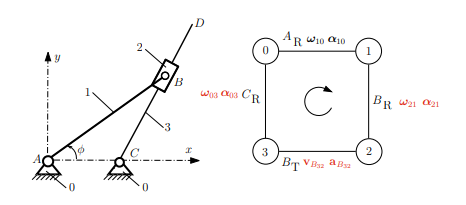
The planar R-RTR mechanism considered in Chap. 2 is shown in Fig. $3.3$ with the attached contour diagram. The input data and the position data are:
$\mathrm{AB}=0.10 ;$ \&ै ${\mathrm{m})$
$\mathrm{AC}=0.05 ;$ \& $(\mathrm{m})$
$C D=0.15 ;$ \& $;(\mathrm{m})$
$\mathrm{phi}=\mathrm{pi} / 6_{i}$ \& \& {rad $\rangle$
$x A=0 ; \quad y A=0 ;$
$r A-\left[\begin{array}{lll}x A & Y A & 0\end{array}\right] ;$
$x C=A C ; Y C=0 ;$
$r C_{-}=[x C y C 0] i$
of $\mathrm{rC}{-}=0.050,0.000,0$ 와 $r \mathrm{~B}{-}=0.087,0.050,0$
of phi2 $=$ phi $3=53.794$ (degrees)
If $\mathrm{rD}{-}=[0.139,0.121,0] \quad(\mathrm{m})$ The mechanism has one contour. The contour is made of $0,1,2,3$, and 0 . A clockwise path is chosen for the contour. The contour has: a rotational joint $R$ between the links 0 and 1 (joint $A{\mathrm{R}}$ ); a rotational joint $\mathrm{R}$ between the links 1 and 2 (joint $B_{\mathrm{R}}$ ); a translational joint $\mathrm{T}$ between the links 2 and 3 (joint $B_{\mathrm{T}}$ ); a rotational joint $\mathrm{R}$ between the links 3 and 0 (joint $C_{\mathrm{R}}$ ). The angular velocity $\omega_{10}$ of the driver link is $\omega_{10}=\omega_{1}=$ $\omega=n \pi / 30=-50 \pi / 30 \mathrm{rad} / \mathrm{s}=-5 \pi / 3 \mathrm{rad} / \mathrm{s}$. The velocity equations for the contour are:
$$
\begin{aligned}
&\boldsymbol{\omega}{10}+\boldsymbol{\omega}{21}+\boldsymbol{\omega}{03}=\mathbf{0}, \ &\mathbf{r}{B} \times \boldsymbol{\omega}{21}+\mathbf{r}{C} \times \boldsymbol{\omega}{03}+\mathbf{v}{B_{3} B_{2}}^{\text {rel }}=\mathbf{0},
\end{aligned}
$$
where $\mathbf{r}{B}=x{B} \mathbf{1}+y_{B} \mathbf{J}, \mathbf{r}{C}=x{C} \mathbf{1}+y_{C} \mathbf{J}$, and
$$
\begin{aligned}
&\boldsymbol{\omega}{10}=\omega{10} \mathbf{k}, \boldsymbol{\omega}{21}=\omega{21} \mathbf{k}, \boldsymbol{\omega}{03}=\omega{03} \mathbf{k} \
&\mathbf{v}{B{3} B_{2}}^{\text {rel }}=\mathbf{v}{B{22}}=v_{B_{12}} \cos \phi_{2} \mathbf{1}+v_{B_{32}} \sin \phi_{2} \mathbf{J}
\end{aligned}
$$
The relative angular velocities $\omega_{21}, \omega_{03}$, and relative linear velocity $v_{B_{22}}$ are the unknowns. Equation (3.18) can be written as
$$
\left[\begin{array}{ccc}
\mathbf{1} & \mathbf{J} & \mathbf{k} \
x_{B} & y_{B} & 0 \
0 & 0 & \omega_{21}
\end{array}\right]+\left[\begin{array}{ccc}
\mathbf{1} & \mathbf{J} & \mathbf{k} \
x_{C} & y_{C} & 0 \
0 & 0 & \omega_{03}
\end{array}\right]+v_{B_{32}} \cos \phi_{2} \mathbf{1}+v_{B_{32}} \sin \phi_{2} \mathbf{J}=\mathbf{0} .
$$
Equation (3.19) represents a system of 3 algebraic equations with 3 unknowns and can be written in MATLAB as:
$$
\begin{aligned}
&n=-50 \ldots ; \text { \& }(\mathrm{rpm}) \
&\text { omega1 }=\left[\begin{array}{ll}
0 & \left.0 \mathrm{pi}{ }^{} \mathrm{n} / 30\right] ; \text { 영 } \end{array} \quad(\mathrm{rad} / \mathrm{s})\right. \end{aligned} $$ of symbolic unknowns syms omega2 $1 \mathrm{z}$ omega03z vB32 omega10_ = omega1_i omega21v_ $=\left[\begin{array}{ll}0 & 0 \text { omega21z}\end{array}\right]$; omega03v $=\left[\begin{array}{ll}0 & 0 \text { omega03z }\end{array}\right]$; $v 32 v_{-}=v B 32^{}[\cos (p h i 2) \sin (p h i 2) \quad 0] ;$
eqlomega_ $=$ omegalo $1_{-}+$omega $21 v_{-}+$omega03v_;
数学代写|matlab仿真代写simulation代做|Force Analysis for R-RTR Mechanism
The inertia forces and moments and the gravity forces on links 2 and 3 are shown in Fig. 3.4a. The input data for joint force analysis are:
동 $r C_{-}=[0.050,0.000,0]$ (m)
뭉 $\mathrm{rB}=[0.087,0.050,0]$ (m)
뭉 phiz $=$ phis $=53.794$ (degrees)
뭉 $\mathrm{rD}{-}=[0.139,0.121,0] \mathrm{(m)}$ 당 $\mathrm{rCl}{-}=[0.043,0.025,0]$ (m)
당 $\mathrm{rC}{-}=[0.087,0.050,0] \mathrm{(m)}$ 당 $\mathrm{rC3}{-}=[0.094,0.061,0]$ (m)
당 $\mathrm{aCl}{-}=[-1.187,-0.685,0]\left(\mathrm{m} / \mathrm{s}^{A} 2\right)$ 당 $a C^{2}=[-2.374,-1.371,0]\left(\mathrm{m} / \mathrm{s}^{A} 2\right)$ 닿 $\mathrm{aC}{3}=[-0.538,-5.162,0]\left(\mathrm{m} / \mathrm{s}^{A} 2\right)$
웅 alpha1 $=[0,0,0.000]\left(\mathrm{rad} / \mathrm{s}^{4} 2\right)$
닿 alpha2 $=[0,0,-34.865]\left(\mathrm{rad} / \mathrm{s}^{4} 2\right)$
당 alpha3 ${ }^{3}=[0,0,-34.865]\left(\mathrm{rad} / \mathrm{s}^{\wedge} 2\right)$
망
당 $\mathrm{Gl}{-}=-\mathrm{m} 1 \mathrm{~g}{-}=[0,-0.078,0] \quad(\mathrm{N})$
닿 Fin1 $=-\mathrm{m} 1 \mathrm{aC1}=[0.009,0.005,0]$ (N)
망 Min1 $=-I C 1$ alpha1 $=[0,0,0](\mathrm{N} \mathrm{m})$
망
왛 $\mathrm{G}{-}=-\mathrm{m} 2 \mathrm{~g}{-}=[0,-0.063,0] \quad(\mathrm{N})$
of $\operatorname{Fin} 2_{-}=-\mathrm{m} 2 \mathrm{aC2}=[0.015,0.009,0] \quad$ (N)
of Min2 $=-I C 2$ alpha2 $2=[0,0,3.719 \mathrm{e}-05](\mathrm{N} \mathrm{m})$
앙
왕 $\mathrm{G}{-}=-\mathrm{m} 3 \mathrm{~g}{-}=0,-0.118,0$
왛 $\mathrm{Fin}{3}=-\mathrm{m} 3 \mathrm{aC3}=[0.006,0.062,0]$ (N) 망 $\operatorname{Min} 3$ $=-\operatorname{IC3}$ alpha3 $=[0,0,7.880 \mathrm{e}-04](\mathrm{N} \mathrm{m})$
of $\mathrm{Me}=[0,0,100.000]$ (N m)
To calculate the joint reaction $\mathbf{F}{03}$ with the application point at the rotational joint $C$ the diagram shown in Fig. 3.4(b) is used. For the link 3, the joint reaction force $\mathbf{F}{23}$ is eliminated if the sum of the forces on link 3 are dot multiplied with the direction of the link $B C$ :
syms F03x F03y
F03_ $=[F 03 x, F 03 y, 0]$; 뫄 unknown joint force of 0 on 3 at $C$
돵 for joint B translation
뭉 $\left(\mathrm{FO} 3_{-}+\mathrm{G} 3_{-}+\mathrm{Fin} 3_{-}+\mathrm{F} 23_{-}\right) \cdot\left(\mathrm{rB}-\mathrm{rC}{-}\right)=0$ 망 $\mathrm{F} 23$ – perpendicular to $\mathrm{BC}$ : $\mathrm{F3} 2{-} \cdot \mathrm{BC}{-}=0$ => eqF3 = $\left(\mathrm{FO} 3{-}+\mathrm{G} 3_{-}+\mathrm{Fin} 3_{-}\right) *\left(\mathrm{rB}-{ }{-} \mathrm{C}{-}\right) \cdot \prime ;$ o $(\mathrm{F} 1)$
matlab代写
数学代写|matlab仿真代写simulation代做|Closed Contour Equations
本研究旨在提供一种代数方法来计算闭合运动链的速度[3,18,71]. 独立轮廓(环)方程的方法非常有效,可以应用于平面和空间力学系统。
考虑两个刚体(j)和(ķ)由关节或运动对连接在一种. 速度之间存在以下关系在一种点的一种j和速度在一种ķ点的一种ķ
在一种j=在一种ķ+在一种jķ,r
在哪里在一种jķr=在一种j一种ķr=在一种j一种ķ是速度一种j正如观察员所见一种ķ附着在身体上(ķ)或相对速度一种j关于一种ķ, 允许在关节处一种. 的加速度一种j和一种ķ表示为
一种一种j=一种一种ķ+一种一种jķr+一种一种jķC,
在哪里一种一种jķr=一种一种j一种ķr=一种一种j一种ķ是相对加速度一种j关于一种ķ和一种一种jķC=一种一种j一种ķCķ是由下式给出的科里奥利加速度
一种一种jķC=2ωķ×在一种jķr,
在哪里ωķ是物体的角速度(ķ). 方程 (3.1) 和 (3.2) 即使对于属于两个可能不直接存在的刚体的重合点也是有用的
连接的。数字3.1显示了一个单环闭合运动链n刚性链接。关节一种一世在哪里一世=1,2,…,n是链接之间的连接(一世)和(一世−1). 在联合处一种一世有两个瞬间重合的点。重点一种一世,一世属于链接(一世),一种一世,一世∈(一世)和重点一种一世,一世−1属于身体(一世−1),一种一世,一世−1∈(一世−1). 刚体的绝对角速度 (一世) 是
ω一世=ω一世−1+ω一世,一世−1
在哪里ω一世,一世−1是刚体 (i) 相对于刚体的相对角速度(一世−1). 为了n连接闭合运动链 角速度方程为ω1=ωn+ω1,n:ω2=ω1+ω2,1:…ω一世=ω一世−1+ω一世,一世−1:…ωn=ωn−1+ωn,n−1 (3.5) 对等式中的表达式求和。(3.5) 得到以下关系ω1,n+ω2,1+…+ωn,n−1=0 或者 ∑(一世)ω一世,一世−1=0
简单闭合运动链的角速度的第一个矢量方程由方程给出。(3.6)。
数学代写|matlab仿真代写simulation代做|Closed Contour Equations for R-RTR Mechanism
第 1 章中考虑的平面 R-RTR 机制。2如图所示。3.3附等高线图。输入数据和位置数据为:
一种乙=0.10;\ & ै $ \ mathrm {m})\数学{AC} = 0.05;&(\数学{m})光盘=0.15;&; (\mathrm {m})\ mathrm {phi} = \ mathrm {pi} / 6_ {i} $ \ & \ & {rad⟩
X一种=0;是一种=0;
r一种−[X一种是一种0];
XC=一种C;是C=0;
rC−=[XC是C0]一世
$\mathrm{rC}{-}= 0.050,0.000,0와哇r \ mathrm ~~ B {-} = 0.087,0.050,0这FpH一世2=pH一世3=53.794(d和Gr和和s)一世F\mathrm{rD}{-}=[0.139,0.121,0] \quad(\mathrm{m})吨H和米和CH一种n一世s米H一种s这n和C这n吨这在r.吨H和C这n吨这在r一世s米一种d和这F0,1,2,3,一种nd0.一种Cl这Cķ在一世s和p一种吨H一世sCH这s和nF这r吨H和C这n吨这在r.吨H和C这n吨这在rH一种s:一种r这吨一种吨一世这n一种lj这一世n吨Rb和吨在和和n吨H和l一世nķs0一种nd1(j这一世n吨A {\ mathrm {R});一种r这吨一种吨一世这n一种lj这一世n吨\数学{Rb和吨在和和n吨H和l一世nķs1一种nd2(j这一世n吨B_{\数学{R});一种吨r一种nsl一种吨一世这n一种lj这一世n吨\mathrm{T}b和吨在和和n吨H和l一世nķs2一种nd3(j这一世n吨B_{\mathrm{T}});一种r这吨一种吨一世这n一种lj这一世n吨\数学{Rb和吨在和和n吨H和l一世nķs3一种nd0(j这一世n吨C_{\数学{R}).吨H和一种nG在l一种r在和l这C一世吨是\omega_{10}这F吨H和dr一世在和rl一世nķ一世s\omega_{10}=\omega_{1}=\ omega = n \ pi / 30 = -50 \ pi / 30 \ mathrm {rad} / \ mathrm {s} = – 5 \ pi / 3 \ mathrm {rad} / \ mathrm {s.吨H和在和l这C一世吨是和q在一种吨一世这nsF这r吨H和C这n吨这在r一种r和:ω10+ω21+ω03=0, r乙×ω21+rC×ω03+在乙3乙2相对 =0,在H和r和\mathbf{r}{B}=x{B} \mathbf{1}+y_{B} \mathbf{J}, \mathbf{r}{C}=x{C} \mathbf{1}+y_{ C} \mathbf{J},一种ndω10=ω10ķ,ω21=ω21ķ,ω03=ω03ķ 在乙3乙2相对 =在乙22=在乙12因φ21+在乙32罪φ2Ĵ吨H和r和l一种吨一世在和一种nG在l一种r在和l这C一世吨一世和s\omega_{21},\omega_{03},一种ndr和l一种吨一世在和l一世n和一种r在和l这C一世吨是v_{B_{22}}一种r和吨H和在nķn这在ns.和q在一种吨一世这n(3.18)C一种nb和在r一世吨吨和n一种s[1Ĵķ X乙是乙0 00ω21]+[1Ĵķ XC是C0 00ω03]+在乙32因φ21+在乙32罪φ2Ĵ=0.和q在一种吨一世这n(3.19)r和pr和s和n吨s一种s是s吨和米这F3一种lG和br一种一世C和q在一种吨一世这ns在一世吨H3在nķn这在ns一种ndC一种nb和在r一世吨吨和n一世n米一种吨大号一种乙一种s:영n=−50…; \& (rp米) 欧米茄1 =[00p一世n/30]; 零 (r一种d/s)这Fs是米b这l一世C在nķn这在nss是米s这米和G一种21 \mathrm{z}omega03z vB32 omega10_ = omega1_i omega21v_omega03z vB32 omega10_ = omega1_i omega21v_=\左[00 欧米茄21z\对];这米和G一种03在=\左[00 omega03z \对];v 32 v_{-}=v B 32^{}[\cos (phi 2) \sin (phi 2) \quad 0] ;eqlomega_eqlomega_=这米和G一种l这1_{-}+这米和G一种21 v _ {-} + $ omega03v_;
数学代写|matlab仿真代写simulation代做|Force Analysis for R-RTR Mechanism
连杆 2 和 3 上的惯性力和力矩以及重力如图 3.4a 所示。关节力分析的输入数据为:
동rC−=[0.050,0.000,0](m)
绿r乙=[0.087,0.050,0](m)
뭉 phiz=菲斯=53.794(度)
뭉rD−=[0.139,0.121,0](米)聚会rCl−=[0.043,0.025,0](m)
每rC−=[0.087,0.050,0](米)聚会rC3−=[0.094,0.061,0](m)
每一种Cl−=[−1.187,−0.685,0](米/s一种2)聚会一种C2=[−2.374,−1.371,0](米/s一种2)到达一种C3=[−0.538,−5.162,0](米/s一种2)
熊阿尔法1=[0,0,0.000](r一种d/s42)
触动了 alpha2=[0,0,−34.865](r一种d/s42)
每个 alpha33=[0,0,−34.865](r一种d/s∧2)
每人
_Gl−=−米1 G−=[0,−0.078,0](ñ)
触动鳍1=−米1一种C1=[0.009,0.005,0](N)
净最小值1=−一世C1阿尔法1=[0,0,0](ñ米)男人摇摆G−=−米2 G−=[0,−0.063,0](ñ)
的结尾2−=−米2一种C2=[0.015,0.009,0](N)
的 Min2=−一世C2阿尔法22=[0,0,3.719和−05](ñ米)
앙
왕 $ \ mathrm {G} {-} = – \ mathrm {m} 3 \ mathrm ~ g {-} = 0, -0.118,0왛哇\ mathrm {Fin} {3} = – \ mathrm {m} 3 \ mathrm {aC3} = [0.006,0.062,0]망(ñ)网\operatorname{Min} 3=-\运营商名称{IC3}一种lpH一种3= [0,0,7.880 \ mathrm {e} -04] (\ mathrm {N} \ mathrm {m})这F\mathrm{我}=[0,0,100.000]$ (N m)
计算联合反应F03在旋转关节处的应用点C使用图 3.4(b) 所示的图表。对于连杆 3,关节反作用力F23如果连杆 3 上的力的总和乘以连杆的方向,则消除乙C:
syms F03x F03y
F03_=[F03X,F03是,0]; 뫄 0 对 3 的未知联合力C
돵 联合 B 翻译
뭉(F这3−+G3−+F一世n3−+F23−)⋅(r乙−rC−)=0网F23– 垂直于乙C : F32−⋅乙C−=0=> eqF3 =(F这3−+G3−+F一世n3−)∗(r乙−−C−)⋅′;这(F1)

统计代写请认准statistics-lab™. statistics-lab™为您的留学生涯保驾护航。
金融工程代写
金融工程是使用数学技术来解决金融问题。金融工程使用计算机科学、统计学、经济学和应用数学领域的工具和知识来解决当前的金融问题,以及设计新的和创新的金融产品。
非参数统计代写
非参数统计指的是一种统计方法,其中不假设数据来自于由少数参数决定的规定模型;这种模型的例子包括正态分布模型和线性回归模型。
广义线性模型代考
广义线性模型(GLM)归属统计学领域,是一种应用灵活的线性回归模型。该模型允许因变量的偏差分布有除了正态分布之外的其它分布。
术语 广义线性模型(GLM)通常是指给定连续和/或分类预测因素的连续响应变量的常规线性回归模型。它包括多元线性回归,以及方差分析和方差分析(仅含固定效应)。
有限元方法代写
有限元方法(FEM)是一种流行的方法,用于数值解决工程和数学建模中出现的微分方程。典型的问题领域包括结构分析、传热、流体流动、质量运输和电磁势等传统领域。
有限元是一种通用的数值方法,用于解决两个或三个空间变量的偏微分方程(即一些边界值问题)。为了解决一个问题,有限元将一个大系统细分为更小、更简单的部分,称为有限元。这是通过在空间维度上的特定空间离散化来实现的,它是通过构建对象的网格来实现的:用于求解的数值域,它有有限数量的点。边界值问题的有限元方法表述最终导致一个代数方程组。该方法在域上对未知函数进行逼近。[1] 然后将模拟这些有限元的简单方程组合成一个更大的方程系统,以模拟整个问题。然后,有限元通过变化微积分使相关的误差函数最小化来逼近一个解决方案。
tatistics-lab作为专业的留学生服务机构,多年来已为美国、英国、加拿大、澳洲等留学热门地的学生提供专业的学术服务,包括但不限于Essay代写,Assignment代写,Dissertation代写,Report代写,小组作业代写,Proposal代写,Paper代写,Presentation代写,计算机作业代写,论文修改和润色,网课代做,exam代考等等。写作范围涵盖高中,本科,研究生等海外留学全阶段,辐射金融,经济学,会计学,审计学,管理学等全球99%专业科目。写作团队既有专业英语母语作者,也有海外名校硕博留学生,每位写作老师都拥有过硬的语言能力,专业的学科背景和学术写作经验。我们承诺100%原创,100%专业,100%准时,100%满意。
随机分析代写
随机微积分是数学的一个分支,对随机过程进行操作。它允许为随机过程的积分定义一个关于随机过程的一致的积分理论。这个领域是由日本数学家伊藤清在第二次世界大战期间创建并开始的。
时间序列分析代写
随机过程,是依赖于参数的一组随机变量的全体,参数通常是时间。 随机变量是随机现象的数量表现,其时间序列是一组按照时间发生先后顺序进行排列的数据点序列。通常一组时间序列的时间间隔为一恒定值(如1秒,5分钟,12小时,7天,1年),因此时间序列可以作为离散时间数据进行分析处理。研究时间序列数据的意义在于现实中,往往需要研究某个事物其随时间发展变化的规律。这就需要通过研究该事物过去发展的历史记录,以得到其自身发展的规律。
回归分析代写
多元回归分析渐进(Multiple Regression Analysis Asymptotics)属于计量经济学领域,主要是一种数学上的统计分析方法,可以分析复杂情况下各影响因素的数学关系,在自然科学、社会和经济学等多个领域内应用广泛。
MATLAB代写
MATLAB 是一种用于技术计算的高性能语言。它将计算、可视化和编程集成在一个易于使用的环境中,其中问题和解决方案以熟悉的数学符号表示。典型用途包括:数学和计算算法开发建模、仿真和原型制作数据分析、探索和可视化科学和工程图形应用程序开发,包括图形用户界面构建MATLAB 是一个交互式系统,其基本数据元素是一个不需要维度的数组。这使您可以解决许多技术计算问题,尤其是那些具有矩阵和向量公式的问题,而只需用 C 或 Fortran 等标量非交互式语言编写程序所需的时间的一小部分。MATLAB 名称代表矩阵实验室。MATLAB 最初的编写目的是提供对由 LINPACK 和 EISPACK 项目开发的矩阵软件的轻松访问,这两个项目共同代表了矩阵计算软件的最新技术。MATLAB 经过多年的发展,得到了许多用户的投入。在大学环境中,它是数学、工程和科学入门和高级课程的标准教学工具。在工业领域,MATLAB 是高效研究、开发和分析的首选工具。MATLAB 具有一系列称为工具箱的特定于应用程序的解决方案。对于大多数 MATLAB 用户来说非常重要,工具箱允许您学习和应用专业技术。工具箱是 MATLAB 函数(M 文件)的综合集合,可扩展 MATLAB 环境以解决特定类别的问题。可用工具箱的领域包括信号处理、控制系统、神经网络、模糊逻辑、小波、仿真等。