如果你也在 怎样代写流体力学Fluid Mechanics这个学科遇到相关的难题,请随时右上角联系我们的24/7代写客服。
流体力学是物理学的一个分支,涉及流体(液体、气体和等离子体)的力学和对它们的力。它的应用范围很广,包括机械、土木工程、化学和生物医学工程、地球物理学、海洋学、气象学、天体物理学和生物学。
statistics-lab™ 为您的留学生涯保驾护航 在代写流体力学Fluid Mechanics方面已经树立了自己的口碑, 保证靠谱, 高质且原创的统计Statistics代写服务。我们的专家在代写流体力学Fluid Mechanics代写方面经验极为丰富,各种代写流体力学Fluid Mechanics相关的作业也就用不着说。
我们提供的流体力学Fluid Mechanics及其相关学科的代写,服务范围广, 其中包括但不限于:
- Statistical Inference 统计推断
- Statistical Computing 统计计算
- Advanced Probability Theory 高等概率论
- Advanced Mathematical Statistics 高等数理统计学
- (Generalized) Linear Models 广义线性模型
- Statistical Machine Learning 统计机器学习
- Longitudinal Data Analysis 纵向数据分析
- Foundations of Data Science 数据科学基础
物理代写|流体力学代写Fluid Mechanics代考|Material and Spatial Descriptions
Kinematics is the study of the motion of a fluid, without considering the forces which cause this motion, that is without considering the equations of motion. It is natural to try to carry over the kinematics of a mass-point directly to the kinematics of a fluid particle. Its motion is given by the time dependent position vector $\vec{x}(t)$ relative to a chosen origin.
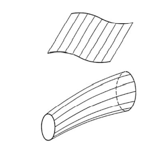
In general we are interested in the motion of a finitely large part of the fluid (or the whole fluid) and this is made up of infinitely many fluid particles. Thus the single particles must remain identifiable. The shape of the particle is no use as an identification, since, because of its ability to deform without limit, it continually changes during the course of the motion. Naturally the linear measure must remain small in spite of the deformation during the motion, something that we guarantee by idealizing the fluid particle as a material point.
For identification, we associate with each material point a characteristic vector $\vec{\xi}$. The position vector $\vec{x}$ at a certain time $t_{0}$ could be chosen, giving $\vec{x}\left(t_{0}\right)=\vec{\xi}$. The motion of the whole fluid can then be described by
$$
\vec{x}=\vec{x}(\vec{\xi}, t) \quad \text { or } \quad x_{i}=x_{i}\left(\xi_{j}, t\right)
$$
物理代写|流体力学代写Fluid Mechanics代考|Pathlines, Streamlines, Streaklines
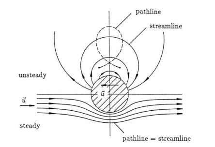
The differential Eq. (1.10) shows that the path of a point in the material is always tangential to its velocity. In this interpretation the pathline is the tangent curve to the velocities of the same material point at different times. Time is the curve parameter, and the material coordinate $\vec{\xi}$ is the family parameter.
Just as the pathline is natural to the material description, so the streamline is natural to the Eulerian description. The velocity field assigns a velocity vector to every place $\vec{x}$ at time $t$ and the streamlines are the curves whose tangent directions are the same as the directions of the velocity vectors. The streamlines provide a vivid description of the flow at time t.
If we interpret the streamlines as the tangent curves to the velocity vectors of different particles in the material at the same instant in time we see that there is no connection between pathlines and streamlines, apart from the fact that they may sometimes lie on the same curve.
By the definition of streamlines, the unit vector $\vec{u} /|\vec{u}|$ is equal to the unit tangent vector of the streamline $\vec{\tau}=\mathrm{d} \vec{x} /|\mathrm{d} \vec{x}|=\mathrm{d} \vec{x} / \mathrm{d} s$ where $\mathrm{d} \vec{x}$ is a vector element of the streamline in the direction of the velocity. The differential equation of the streamline then reads
$$
\frac{\mathrm{d} \vec{x}}{\mathrm{~d} s}=\frac{\vec{u}(\vec{x}, t)}{|\vec{u}|}, \quad(t=\text { const })
$$
or in index notation
$$
\frac{\mathrm{d} x_{i}}{\mathrm{~d} s}=\frac{u_{i}\left(x_{j}, t\right)}{\sqrt{u_{k} u_{k}}}, \quad(t=\mathrm{const})
$$
Integration of these equations with the “initial condition” that the streamline emanates from a point in space $\vec{x}{0}\left(\vec{x}(s=0)=\vec{x}{0}\right)$ leads to the parametric representation of the streamline $\vec{x}=\vec{x}\left(s, \vec{x}{0}\right)$. The curve parameter here is the arc length $s$ measured from $x{0}$, and the family parameter is $\dot{x}_{0}$.
物理代写|流体力学代写Fluid Mechanics代考|Differentiation with Respect to Time
In the Eulerian description our attention is directed towards events at the place $\vec{x}$ at time $t$. However the rate of change of the velocity $\vec{u}$ at $\vec{x}$ is not generally the acceleration which the point in the material passing through $\vec{x}$ at time $t$ experiences. This is obvious in the case of steady flows where the rate of change at a given place is zero. Yet a material point experiences a change in velocity (an acceleration) when it moves from $\vec{x}$ to $\vec{x}+\mathrm{d} \vec{x}$. Here $\mathrm{d} \vec{x}$ is the vector element of the pathline. The changes felt by a point of the material or by some larger part of the fluid and not the time changes at a given place or region of space are of fundamental importance in the dynamics. If the velocity (or some other quantity) is given in material coordinates, then the material or substantial derivative is provided by (1.6). But if the velocity is given in field coordinates, the place $\vec{x}$ in $\vec{u}(\vec{x}, t)$ is replaced by the path coordinates of the particle that occupies $\vec{x}$ at time $t$, and the derivative with respect to time at fixed $\vec{\xi}$ can be formed from
$$
\frac{\mathrm{d} \vec{u}}{\mathrm{~d} t}=\left{\frac{\partial \vec{u}{\vec{x}(\vec{\xi}, t), t}}{\partial t}\right}_{\vec{\xi}}
$$
or
$$
\frac{\mathrm{d} u_{i}}{\mathrm{~d} t}=\left{\frac{\partial u_{i}\left{x_{j}\left(\xi_{k}, t\right), t\right}}{\partial t}\right}_{\xi_{k}}
$$
The material derivative in field coordinates can also be found without direct reference to the material coordinates. Take the temperature field $T(\vec{x}, t)$ as an example: we take the total differential to be the expression
$$
\mathrm{d} T=\frac{\partial T}{\partial t} \mathrm{~d} t+\frac{\partial T}{\partial x_{1}} \mathrm{~d} x_{1}+\frac{\partial T}{\partial x_{2}} \mathrm{~d} x_{2}+\frac{\partial T}{\partial x_{3}} \mathrm{~d} x_{3}
$$
The first term on the right-hand side is the rate of change of the temperature at a fixed place: the local change. The other three terms give the change in temperature by advancing from $\vec{x}$ to $\vec{x}+\mathrm{d} \vec{x}$. This is the convective change. The last three terms can be combined to give $\mathrm{d} \vec{x} \cdot \nabla T$ or equivalently $\mathrm{d} x_{i} \partial T / \partial x_{i}$. If $\mathrm{d} \vec{x}$ is the vector element of the fluid particle’s path at $\vec{x}$, then (1.10) holds and the rate of change of the temperature of the particle passing $\vec{x}$ (the material change of the temperature) is
$$
\frac{\mathrm{d} T}{\mathrm{~d} t}=\frac{\partial T}{\partial t}+\vec{u} \cdot \nabla T
$$
or
$$
\frac{\mathrm{d} T}{\mathrm{~d} t}=\frac{\partial T}{\partial t}+u_{i} \frac{\partial T}{\partial x_{i}}=\frac{\partial T}{\partial t}+u_{1} \frac{\partial T}{\partial x_{1}}+u_{2} \frac{\partial T}{\partial x_{2}}+u_{3} \frac{\partial T}{\partial x_{3}}
$$
流体力学代写
物理代写|流体力学代写Fluid Mechanics代考|Material and Spatial Descriptions
运动学是对流体运动的研究,不考虑引起这种运动的力,即不考虑运动方程。尝试将质点的运动学直接传递到流体粒子的运动学是很自然的。它的运动由时间相关的位置向量给出X→(吨)相对于选定的原点。
一般来说,我们对有限大部分流体(或整个流体)的运动感兴趣,它由无限多的流体粒子组成。因此,单个粒子必须保持可识别性。粒子的形状不能用作识别,因为由于它具有无限变形的能力,它在运动过程中不断变化。自然,尽管运动过程中发生变形,线性测量必须保持较小,这是我们通过将流体粒子理想化为质点来保证的。
为了识别,我们将每个材料点与一个特征向量相关联X→. 位置向量X→在某个时间吨0可以选择,给予X→(吨0)=X→. 整个流体的运动可以描述为
X→=X→(X→,吨) 或者 X一世=X一世(Xj,吨)
物理代写|流体力学代写Fluid Mechanics代考|Pathlines, Streamlines, Streaklines
微分方程。(1.10) 表明材料中一点的路径总是与其速度相切。在这种解释中,路径线是同一质点在不同时间的速度的切线。时间为曲线参数,材料坐标X→是家庭参数。
正如路径线对于材料描述来说是自然的一样,流线对于欧拉描述来说也是自然的。速度场为每个位置分配一个速度矢量X→有时吨流线是切线方向与速度矢量方向相同的曲线。流线对时间 t 的流动提供了生动的描述。
如果我们将流线解释为材料中不同粒子在同一时刻的速度矢量的切线曲线,我们会看到路径线和流线之间没有联系,除了它们有时可能位于同一曲线上的事实.
根据流线的定义,单位向量在→/|在→|等于流线的单位切向量τ→=dX→/|dX→|=dX→/ds在哪里dX→是流线在速度方向上的矢量元素。流线的微分方程然后读取
dX→ ds=在→(X→,吨)|在→|,(吨= 常量 )
或以索引表示法
dX一世 ds=在一世(Xj,吨)在ķ在ķ,(吨=C○ns吨)
将这些方程与流线从空间中的一点发出的“初始条件”整合X→0(X→(s=0)=X→0)导致流线的参数化表示X→=X→(s,X→0). 这里的curve参数是弧长s从测量X0, 族参数为X˙0.
物理代写|流体力学代写Fluid Mechanics代考|Differentiation with Respect to Time
在欧拉描述中,我们的注意力集中在该地点的事件上X→有时吨. 然而速度的变化率在→在X→通常不是材料中的点通过的加速度X→有时吨经验。这在给定位置的变化率为零的稳定流的情况下是显而易见的。然而,当一个质点从X→至X→+dX→. 这里dX→是路径的向量元素。材料的一点或流体的较大部分感受到的变化,而不是空间给定位置或区域的时间变化,在动力学中是至关重要的。如果速度(或其他一些量)在材料坐标中给出,则材料或实质导数由 (1.6) 提供。但是如果速度是在场坐标中给出的,那么这个地方X→在在→(X→,吨)替换为占据的粒子的路径坐标X→有时吨,以及关于固定时间的导数X→可以由
\frac{\mathrm{d} \vec{u}}{\mathrm{~d} t}=\left{\frac{\partial \vec{u}{\vec{x}(\vec{\xi} , t), t}}{\partial t}\right}_{\vec{\xi}}\frac{\mathrm{d} \vec{u}}{\mathrm{~d} t}=\left{\frac{\partial \vec{u}{\vec{x}(\vec{\xi} , t), t}}{\partial t}\right}_{\vec{\xi}}
或者
\frac{\mathrm{d} u_{i}}{\mathrm{~d} t}=\left{\frac{\partial u_{i}\left{x_{j}\left(\xi_{k} , t\right), t\right}}{\partial t}\right}_{\xi_{k}}\frac{\mathrm{d} u_{i}}{\mathrm{~d} t}=\left{\frac{\partial u_{i}\left{x_{j}\left(\xi_{k} , t\right), t\right}}{\partial t}\right}_{\xi_{k}}
也可以在不直接参考材料坐标的情况下找到场坐标中的材料导数。取温度场吨(X→,吨)举个例子:我们把总微分作为表达式
d吨=∂吨∂吨 d吨+∂吨∂X1 dX1+∂吨∂X2 dX2+∂吨∂X3 dX3
右边的第一项是固定位置的温度变化率:局部变化。其他三个项通过从前进给出温度变化X→至X→+dX→. 这就是对流变化。最后三个术语可以组合给出dX→⋅∇吨或等效地dX一世∂吨/∂X一世. 如果dX→是流体粒子路径的向量元素X→, 那么 (1.10) 成立并且粒子通过的温度变化率X→(温度的物质变化)是
d吨 d吨=∂吨∂吨+在→⋅∇吨
或者
d吨 d吨=∂吨∂吨+在一世∂吨∂X一世=∂吨∂吨+在1∂吨∂X1+在2∂吨∂X2+在3∂吨∂X3

统计代写请认准statistics-lab™. statistics-lab™为您的留学生涯保驾护航。
金融工程代写
金融工程是使用数学技术来解决金融问题。金融工程使用计算机科学、统计学、经济学和应用数学领域的工具和知识来解决当前的金融问题,以及设计新的和创新的金融产品。
非参数统计代写
非参数统计指的是一种统计方法,其中不假设数据来自于由少数参数决定的规定模型;这种模型的例子包括正态分布模型和线性回归模型。
广义线性模型代考
广义线性模型(GLM)归属统计学领域,是一种应用灵活的线性回归模型。该模型允许因变量的偏差分布有除了正态分布之外的其它分布。
术语 广义线性模型(GLM)通常是指给定连续和/或分类预测因素的连续响应变量的常规线性回归模型。它包括多元线性回归,以及方差分析和方差分析(仅含固定效应)。
有限元方法代写
有限元方法(FEM)是一种流行的方法,用于数值解决工程和数学建模中出现的微分方程。典型的问题领域包括结构分析、传热、流体流动、质量运输和电磁势等传统领域。
有限元是一种通用的数值方法,用于解决两个或三个空间变量的偏微分方程(即一些边界值问题)。为了解决一个问题,有限元将一个大系统细分为更小、更简单的部分,称为有限元。这是通过在空间维度上的特定空间离散化来实现的,它是通过构建对象的网格来实现的:用于求解的数值域,它有有限数量的点。边界值问题的有限元方法表述最终导致一个代数方程组。该方法在域上对未知函数进行逼近。[1] 然后将模拟这些有限元的简单方程组合成一个更大的方程系统,以模拟整个问题。然后,有限元通过变化微积分使相关的误差函数最小化来逼近一个解决方案。
tatistics-lab作为专业的留学生服务机构,多年来已为美国、英国、加拿大、澳洲等留学热门地的学生提供专业的学术服务,包括但不限于Essay代写,Assignment代写,Dissertation代写,Report代写,小组作业代写,Proposal代写,Paper代写,Presentation代写,计算机作业代写,论文修改和润色,网课代做,exam代考等等。写作范围涵盖高中,本科,研究生等海外留学全阶段,辐射金融,经济学,会计学,审计学,管理学等全球99%专业科目。写作团队既有专业英语母语作者,也有海外名校硕博留学生,每位写作老师都拥有过硬的语言能力,专业的学科背景和学术写作经验。我们承诺100%原创,100%专业,100%准时,100%满意。
随机分析代写
随机微积分是数学的一个分支,对随机过程进行操作。它允许为随机过程的积分定义一个关于随机过程的一致的积分理论。这个领域是由日本数学家伊藤清在第二次世界大战期间创建并开始的。
时间序列分析代写
随机过程,是依赖于参数的一组随机变量的全体,参数通常是时间。 随机变量是随机现象的数量表现,其时间序列是一组按照时间发生先后顺序进行排列的数据点序列。通常一组时间序列的时间间隔为一恒定值(如1秒,5分钟,12小时,7天,1年),因此时间序列可以作为离散时间数据进行分析处理。研究时间序列数据的意义在于现实中,往往需要研究某个事物其随时间发展变化的规律。这就需要通过研究该事物过去发展的历史记录,以得到其自身发展的规律。
回归分析代写
多元回归分析渐进(Multiple Regression Analysis Asymptotics)属于计量经济学领域,主要是一种数学上的统计分析方法,可以分析复杂情况下各影响因素的数学关系,在自然科学、社会和经济学等多个领域内应用广泛。
MATLAB代写
MATLAB 是一种用于技术计算的高性能语言。它将计算、可视化和编程集成在一个易于使用的环境中,其中问题和解决方案以熟悉的数学符号表示。典型用途包括:数学和计算算法开发建模、仿真和原型制作数据分析、探索和可视化科学和工程图形应用程序开发,包括图形用户界面构建MATLAB 是一个交互式系统,其基本数据元素是一个不需要维度的数组。这使您可以解决许多技术计算问题,尤其是那些具有矩阵和向量公式的问题,而只需用 C 或 Fortran 等标量非交互式语言编写程序所需的时间的一小部分。MATLAB 名称代表矩阵实验室。MATLAB 最初的编写目的是提供对由 LINPACK 和 EISPACK 项目开发的矩阵软件的轻松访问,这两个项目共同代表了矩阵计算软件的最新技术。MATLAB 经过多年的发展,得到了许多用户的投入。在大学环境中,它是数学、工程和科学入门和高级课程的标准教学工具。在工业领域,MATLAB 是高效研究、开发和分析的首选工具。MATLAB 具有一系列称为工具箱的特定于应用程序的解决方案。对于大多数 MATLAB 用户来说非常重要,工具箱允许您学习和应用专业技术。工具箱是 MATLAB 函数(M 文件)的综合集合,可扩展 MATLAB 环境以解决特定类别的问题。可用工具箱的领域包括信号处理、控制系统、神经网络、模糊逻辑、小波、仿真等。