如果你也在 怎样代写多元统计分析Multivariate Statistical Analysis这个学科遇到相关的难题,请随时右上角联系我们的24/7代写客服。
多变量统计分析被认为是评估地球化学异常与任何单独变量和变量之间相互影响的意义的有用工具。
statistics-lab™ 为您的留学生涯保驾护航 在代写多元统计分析Multivariate Statistical Analysis方面已经树立了自己的口碑, 保证靠谱, 高质且原创的统计Statistics代写服务。我们的专家在代写多元统计分析Multivariate Statistical Analysis代写方面经验极为丰富,各种代写多元统计分析Multivariate Statistical Analysis相关的作业也就用不着说。
我们提供的多元统计分析Multivariate Statistical Analysis及其相关学科的代写,服务范围广, 其中包括但不限于:
- Statistical Inference 统计推断
- Statistical Computing 统计计算
- Advanced Probability Theory 高等概率论
- Advanced Mathematical Statistics 高等数理统计学
- (Generalized) Linear Models 广义线性模型
- Statistical Machine Learning 统计机器学习
- Longitudinal Data Analysis 纵向数据分析
- Foundations of Data Science 数据科学基础
统计代写|多元统计分析代写Multivariate Statistical Analysis代考|KernelParallel Coordinates Plots
PCP is a method for representing high-dimensional data, see Inselberg (1985). Instead of plotting observations in an orthogonal coordinate system, PCP draws coordinates in parallel axes and connects them with straight lines. This method helps in representing data with more than four dimensions.
One first scales all variables to $\max =1$ and $\min =0$. The coordinate index $j$ is drawn onto the horizontal axis, and the scaled value of variable $x_{i j}$ is mapped onto the vertical axis. This way of representation is very useful for high-dimensional data. It is however also sensitive to the order of the variables, since certain trends in the data can be shown more clearly in one ordering than in another.
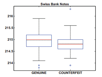
Example 1.5 Take, once again, the observations $96-105$ of the Swiss bank notes. These observations are six dimensional, so we can’t show them in a six-dimensional Cartesian coordinate system. Using the PCP technique, however, they can be plotted on parallel axes. This is shown in Fig. 1.22.
PCP can also be used for detecting linear dependencies between variables: if all the lines are of almost parallel dimensions $(p=2)$, there is a positive linear dependence between them. In Fig. $1.23$ we display the two variables weight and displacement for the car data set in Sect. 22.3. The correlation coefficient $\rho$ introduced in Sect. $3.2$ is $0.9$. If all lines intersect visibly in the middle, there is evidence of a negative linear dependence between these two variables, see Fig. $1.24$. In fact the correlation is $\rho=-0.82$ between two variables mileage and weight: The more the weight, the less the mileage.
统计代写|多元统计分析代写Multivariate Statistical Analysis代考|Hexagon Plots
This section closely follows the presentation of Lewin-Koh (2006). In geometry, a hexagon is a polygon with six edges and six vertices. Hexagon binning is a type of bivariate histogram with hexagon borders. It is useful for visualising the structure of data sets entailing a large number of observations $n$. The concept of hexagon binning is as follows:
- The $x y$ plane over the set (range $(x)$, $\operatorname{range}(y)$ ) is tessellated by a regular grid of hexagons.
- The number of points falling in each hexagon is counted.
- The hexagons with count $>0$ are plotted by using a colour ramp or varying the radius of the hexagon in proportion to the counts.
This algorithm is extremely fast and effective for displaying the structure of data sets even for $n \geq 10^{6}$. If the size of the grid and the cuts in the colour ramp are chosen in a clever fashion, then the structure inherent in the data should emerge in the binned plot. The same caveats apply to hexagon binning as histograms. Variance and bias vary in opposite directions with bin width, so we have to settle for finding the value of the bin width that yields the optimal compromise between variance and bias reduction. Clearly, if we increase the size of the grid, the hexagon plot appears to be smoother, but without some reasonable criterion on hand it remains difficult to say which bin width provides the “optimal” degree of smoothness. The default number of bins suggested by standard software is 30 .
Applications to some data sets are shown as follows. The data is taken from ALLBUS (2006) [ZA No.3762]. The number of respondents is 2,946 . The following nine variables have been selected to analyse the relation between each pair of variables.
统计代写|多元统计分析代写Multivariate Statistical Analysis代考|Quadratic Forms
A quadratic form $Q(x)$ is built from a symmetric matrix $\mathcal{A}(p \times p)$ and a vector $x \in \mathbb{R}^{p}:$
$$
Q(x)=x^{\top}, \mathcal{A} x=\sum_{i=1}^{p} \sum_{j=1}^{p} a_{i j} x_{i} x_{j}
$$
Definiteness of Quadratic Forms and Matrices
$$
\begin{array}{ll}
Q(x)>0 \text { for all } x \neq 0 & \text { positive definite } \
Q(x) \geq 0 \text { for all } x \neq 0 & \text { positive semidefinite }
\end{array}
$$
A matrix $\mathcal{A}$ is called positive definite (semidefinite) if the corresponding quadratic form $Q(.)$ is positive definite (semidefinite). We write $\mathcal{A}>0(\geq 0)$.
Quadratic forms can always be diagonalised, as the following result shows.
Theorem 2.3 If $\mathcal{A}$ is symmetric and $Q(x)=x^{\top} \mathcal{A} x$ is the corresponding quadratic form, then there exists a transformation $x \mapsto \Gamma^{\top} x=y$ such that
$$
x^{\top} \mathcal{A} x=\sum_{i=1}^{p} \lambda_{i} y_{i}^{2}
$$
where $\lambda_{i}$ are the eigenvalues of $\mathcal{A}$.
Proof $\mathcal{A}=\Gamma \Lambda \Gamma^{\top}$. By Theorem $2.1$ and $y=\Gamma^{\top} \alpha$ we have that $x^{\top} \mathcal{A} x=$ $x^{\top} \Gamma \Lambda \Gamma^{\top} x=y^{\top} \Lambda y=\sum_{i=1}^{p} \lambda_{i} y_{i}^{2}$.
Positive definiteness of quadratic forms can be deduced from positive eigenvalues.
Theorem $2.4 \mathcal{A}>0$ if and only if all $\lambda_{i}>0, i=1, \ldots, p$.
Proof $0<\lambda_{1} y_{1}^{2}+\cdots+\lambda_{p} y_{p}^{2}=x^{\top} \mathcal{A} x$ for all $x \neq 0$ by Theorem 2.3.
多元统计分析代考
统计代写|多元统计分析代写Multivariate Statistical Analysis代考|KernelParallel Coordinates Plots
PCP 是一种表示高维数据的方法,参见 Inselberg (1985)。PCP 不是在正交坐标系中绘制观测值,而是在平行轴上绘制坐标并用直线连接它们。此方法有助于表示具有四个以上维度的数据。
首先将所有变量缩放为最大限度=1和分钟=0. 坐标索引j绘制在水平轴上,变量的缩放值X一世j映射到垂直轴上。这种表示方式对于高维数据非常有用。然而,它对变量的顺序也很敏感,因为数据中的某些趋势可以以一种顺序比另一种顺序更清楚地显示。
例 1.5 再次观察观察结果96−105瑞士银行纸币。这些观察是六维的,所以我们不能在六维笛卡尔坐标系中显示它们。然而,使用 PCP 技术,它们可以绘制在平行轴上。如图 1.22 所示。
PCP 也可用于检测变量之间的线性依赖关系:如果所有线的维度几乎平行(p=2),它们之间存在正线性相关。在图。1.23我们显示了 Sect 中汽车数据集的两个变量权重和位移。22.3. 相关系数ρ节中介绍。3.2是0.9. 如果所有线在中间明显相交,则有证据表明这两个变量之间存在负线性相关性,见图。1.24. 实际上相关性是ρ=−0.82里程和重量两个变量之间:重量越大,里程越少。
统计代写|多元统计分析代写Multivariate Statistical Analysis代考|Hexagon Plots
本节紧跟 Lewin-Koh (2006) 的介绍。在几何学中,六边形是一个有六个边和六个顶点的多边形。六边形分箱是一种具有六边形边界的二元直方图。它对于可视化需要大量观察的数据集的结构很有用n. 六边形分箱的概念如下:
- 这X是平面上的集合(范围(X), 范围(是)) 由六边形的规则网格镶嵌。
- 计算落在每个六边形中的点数。
- 有计数的六边形>0通过使用色带或与计数成比例地改变六边形的半径来绘制。
该算法非常快速有效地显示数据集的结构,即使对于n≥106. 如果以巧妙的方式选择网格的大小和色带中的切口,则数据中固有的结构应该出现在分箱图中。相同的注意事项适用于直方图的六边形分箱。方差和偏差随 bin 宽度的变化方向相反,因此我们必须找到在方差和偏差减少之间产生最佳折衷的 bin 宽度值。显然,如果我们增加网格的大小,六边形图看起来会更平滑,但如果没有一些合理的标准,仍然很难说哪个 bin 宽度提供了“最佳”平滑度。标准软件建议的默认 bin 数量为 30 。
一些数据集的应用如下所示。数据取自 ALLBUS (2006) [ZA No.3762]。受访者人数为 2,946 人。选择了以下九个变量来分析每对变量之间的关系。
统计代写|多元统计分析代写Multivariate Statistical Analysis代考|Quadratic Forms
二次形式问(X)由对称矩阵构建一个(p×p)和一个向量X∈Rp:
问(X)=X⊤,一个X=∑一世=1p∑j=1p一个一世jX一世Xj
二次形式和矩阵的确定性
问(X)>0 对所有人 X≠0 正定 问(X)≥0 对所有人 X≠0 正半定
矩阵一个如果对应的二次型称为正定(半定)问(.)是正定(半定)。我们写一个>0(≥0).
二次形式总是可以对角化,如下面的结果所示。
定理 2.3 如果一个是对称的并且问(X)=X⊤一个X是对应的二次型,则存在变换X↦Γ⊤X=是这样
X⊤一个X=∑一世=1pλ一世是一世2
在哪里λ一世是的特征值一个.
证明一个=ΓΛΓ⊤. 按定理2.1和是=Γ⊤一个我们有X⊤一个X= X⊤ΓΛΓ⊤X=是⊤Λ是=∑一世=1pλ一世是一世2.
二次形式的正定性可以从正特征值推导出来。
定理2.4一个>0当且仅当所有λ一世>0,一世=1,…,p.
证明0<λ1是12+⋯+λp是p2=X⊤一个X对所有人X≠0由定理 2.3。

统计代写请认准statistics-lab™. statistics-lab™为您的留学生涯保驾护航。
金融工程代写
金融工程是使用数学技术来解决金融问题。金融工程使用计算机科学、统计学、经济学和应用数学领域的工具和知识来解决当前的金融问题,以及设计新的和创新的金融产品。
非参数统计代写
非参数统计指的是一种统计方法,其中不假设数据来自于由少数参数决定的规定模型;这种模型的例子包括正态分布模型和线性回归模型。
广义线性模型代考
广义线性模型(GLM)归属统计学领域,是一种应用灵活的线性回归模型。该模型允许因变量的偏差分布有除了正态分布之外的其它分布。
术语 广义线性模型(GLM)通常是指给定连续和/或分类预测因素的连续响应变量的常规线性回归模型。它包括多元线性回归,以及方差分析和方差分析(仅含固定效应)。
有限元方法代写
有限元方法(FEM)是一种流行的方法,用于数值解决工程和数学建模中出现的微分方程。典型的问题领域包括结构分析、传热、流体流动、质量运输和电磁势等传统领域。
有限元是一种通用的数值方法,用于解决两个或三个空间变量的偏微分方程(即一些边界值问题)。为了解决一个问题,有限元将一个大系统细分为更小、更简单的部分,称为有限元。这是通过在空间维度上的特定空间离散化来实现的,它是通过构建对象的网格来实现的:用于求解的数值域,它有有限数量的点。边界值问题的有限元方法表述最终导致一个代数方程组。该方法在域上对未知函数进行逼近。[1] 然后将模拟这些有限元的简单方程组合成一个更大的方程系统,以模拟整个问题。然后,有限元通过变化微积分使相关的误差函数最小化来逼近一个解决方案。
tatistics-lab作为专业的留学生服务机构,多年来已为美国、英国、加拿大、澳洲等留学热门地的学生提供专业的学术服务,包括但不限于Essay代写,Assignment代写,Dissertation代写,Report代写,小组作业代写,Proposal代写,Paper代写,Presentation代写,计算机作业代写,论文修改和润色,网课代做,exam代考等等。写作范围涵盖高中,本科,研究生等海外留学全阶段,辐射金融,经济学,会计学,审计学,管理学等全球99%专业科目。写作团队既有专业英语母语作者,也有海外名校硕博留学生,每位写作老师都拥有过硬的语言能力,专业的学科背景和学术写作经验。我们承诺100%原创,100%专业,100%准时,100%满意。
随机分析代写
随机微积分是数学的一个分支,对随机过程进行操作。它允许为随机过程的积分定义一个关于随机过程的一致的积分理论。这个领域是由日本数学家伊藤清在第二次世界大战期间创建并开始的。
时间序列分析代写
随机过程,是依赖于参数的一组随机变量的全体,参数通常是时间。 随机变量是随机现象的数量表现,其时间序列是一组按照时间发生先后顺序进行排列的数据点序列。通常一组时间序列的时间间隔为一恒定值(如1秒,5分钟,12小时,7天,1年),因此时间序列可以作为离散时间数据进行分析处理。研究时间序列数据的意义在于现实中,往往需要研究某个事物其随时间发展变化的规律。这就需要通过研究该事物过去发展的历史记录,以得到其自身发展的规律。
回归分析代写
多元回归分析渐进(Multiple Regression Analysis Asymptotics)属于计量经济学领域,主要是一种数学上的统计分析方法,可以分析复杂情况下各影响因素的数学关系,在自然科学、社会和经济学等多个领域内应用广泛。
MATLAB代写
MATLAB 是一种用于技术计算的高性能语言。它将计算、可视化和编程集成在一个易于使用的环境中,其中问题和解决方案以熟悉的数学符号表示。典型用途包括:数学和计算算法开发建模、仿真和原型制作数据分析、探索和可视化科学和工程图形应用程序开发,包括图形用户界面构建MATLAB 是一个交互式系统,其基本数据元素是一个不需要维度的数组。这使您可以解决许多技术计算问题,尤其是那些具有矩阵和向量公式的问题,而只需用 C 或 Fortran 等标量非交互式语言编写程序所需的时间的一小部分。MATLAB 名称代表矩阵实验室。MATLAB 最初的编写目的是提供对由 LINPACK 和 EISPACK 项目开发的矩阵软件的轻松访问,这两个项目共同代表了矩阵计算软件的最新技术。MATLAB 经过多年的发展,得到了许多用户的投入。在大学环境中,它是数学、工程和科学入门和高级课程的标准教学工具。在工业领域,MATLAB 是高效研究、开发和分析的首选工具。MATLAB 具有一系列称为工具箱的特定于应用程序的解决方案。对于大多数 MATLAB 用户来说非常重要,工具箱允许您学习和应用专业技术。工具箱是 MATLAB 函数(M 文件)的综合集合,可扩展 MATLAB 环境以解决特定类别的问题。可用工具箱的领域包括信号处理、控制系统、神经网络、模糊逻辑、小波、仿真等。