如果你也在 怎样代写强化学习Reinforcement Learning这个学科遇到相关的难题,请随时右上角联系我们的24/7代写客服。
强化学习是一种基于奖励期望行为和/或惩罚不期望行为的机器学习训练方法。一般来说,强化学习代理能够感知和解释其环境,采取行动并通过试验和错误学习。
statistics-lab™ 为您的留学生涯保驾护航 在代写强化学习Reinforcement Learning方面已经树立了自己的口碑, 保证靠谱, 高质且原创的统计Statistics代写服务。我们的专家在代写强化学习Reinforcement Learning代写方面经验极为丰富,各种代写强化学习Reinforcement Learning相关的作业也就用不着说。
我们提供的强化学习Reinforcement Learning及其相关学科的代写,服务范围广, 其中包括但不限于:
- Statistical Inference 统计推断
- Statistical Computing 统计计算
- Advanced Probability Theory 高等楖率论
- Advanced Mathematical Statistics 高等数理统计学
- (Generalized) Linear Models 广义线性模型
- Statistical Machine Learning 统计机器学习
- Longitudinal Data Analysis 纵向数据分析
- Foundations of Data Science 数据科学基础
统计代写|强化学习作业代写Reinforcement Learning代考|On-Policy SARSA
Like the MC control methods, we will again leverage GPI. We will use a TD-driven approach for the policy value estimation/prediction step and will continue to use greedy maximization for the policy improvement. Just like with $\mathrm{MC}$, we need to explore enough and visit all the states an infinite number of times to find an optimal policy. Similar to the MC method, we can use a $\varepsilon$-greedy policy and slowly reduce the $\varepsilon$ value to zero, i.e., for the limit bring down the exploration to zero.
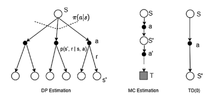
TD setup is model-free; i.e., we have no prior comprehensive knowledge of transitions. At the same time, to be able to maximize the return by choosing the right actions, we need to know the state-action values $Q(S, A)$. We can reformulate TD estimation from equation (4.4) to the one in (4.6), essentially replacing $V(s)$ with $Q(s, a)$. Both the setups are Markov processes, with equation (4.4) focusing on state-to-state transitions and now the focus being state-action to state-action.
$$
Q\left(S_{t}, A_{t}\right)=Q\left(S_{t}, A_{t}\right)+\alpha *\left[R_{t+1}+\gamma * Q\left(S_{t+1}, A_{t+1}\right)-Q\left(S_{t}, A_{t}\right)\right]
$$
Similar to equation (4.5), the TD error is now given in context of q-values.
$$
\delta_{t}=R_{t+1}+\gamma * Q\left(S_{t+1}, A_{t+1}\right)-Q\left(S_{t}, A_{t}\right)
$$
To carry out an update as per equation (4.6), we need all the five values $S_{t}, A_{t} R_{t+1}$, $S_{t+1}$, and $A_{t+1}$. This is the reason the approach is called SARSA (state, action, reward, state, action). We will follow a $\varepsilon$-greedy policy to generate the samples, update the q-values using (4.6), and then based on the updated q-values create a new $\varepsilon$-greedy. The policy improvement theorem guarantees that the new policy will be better than the old policy unless the old policy was already optimal. Of course, for the guarantee to hold, we need to bring down the exploration probability $\varepsilon$ to zero in the limit.
Please also note that for all episodic policies, the terminal states have $Q(S, A)$ equal to zero; i.e., once in terminal state, the person cannot transition anywhere and will keep getting a reward of zero. This is another way of saying that the episode ends and $Q(S, A)$ is zero for all terminal states. Therefore, when $S_{t+1}$ is a terminal state, equation (4.6) will have $Q\left(S_{t+1}, A_{t+1}\right)=0$, and the update equation will look like this:
$$
Q\left(S_{t}, A_{t}\right)=Q\left(S_{t}, A_{t}\right)+\alpha *\left[R_{t+1}-Q\left(S_{t}, A_{t}\right)\right]
$$
Let’s now look at the pseudocode of the SARSA algorithm; see Figure 4-13.
统计代写|强化学习作业代写Reinforcement Learning代考|An Off-Policy TD Control
In SARSA, we used the samples with the values $S, A, R, S^{\prime}$, and $A^{\prime}$ that were generated by the following policy. Action $A^{\prime}$ from state $S^{\prime}$ was produced using the $\varepsilon$-greedy policy, the same policy that was then improved in the “improvement” step of GPI. However, instead of generating $A^{\prime}$ from the policy, what if we looked at all the $Q\left(S, A^{\prime}\right)$ and chose the action $A^{\prime}$, which maximizes the value of $\mathrm{Q}\left(\mathrm{S}^{\prime}, \mathrm{A}^{\prime}\right)$ across actions $A^{\prime}$ available in state $S^{\prime}$ ? We could continue to generate the samples $\left(S, A, R, S^{\prime}\right.$ ) (notice no $A^{\prime}$ as the fifth value in this tuple) using an exploratory policy like $\varepsilon$-greedy. However, we improve the policy by choosing $A^{\prime}$ to be $\operatorname{argmax}{A} Q\left(S, A^{\prime}\right)$. This small change in the approach creates a new way to learn the optimal policy called $Q$-learning. It is no more an on-policy learning, rather an off-policy control method where the samples $\left(S, A, R, S^{\prime}\right)$ are being generated by an exploratory policy, while we maximize $Q\left(S^{\prime}, A\right)$ to find a deterministic optimal target policy. We are using exploration with the $\varepsilon$-greedy policy to generate the samples $(S, A, R, S)$. At the same time, we are exploiting the existing knowledge by finding the $\mathrm{Q}$ maximizing action $\operatorname{argmax}{A} \cdot Q\left(S^{\prime}, A^{\prime}\right)$ in state $S^{\prime}$. We will have lot more to say about these trade-offs between exploration and exploitation in Chapter $9 .$
The update rule for $\mathrm{q}$-values is now defined as follows:
$$
Q\left(S_{t}, A_{t}\right) \leftarrow Q\left(S_{t}, A_{t}\right)+\alpha *\left[R_{t+1}+\gamma * \max {A{t+1}} Q\left(S_{t+1}, A_{t+1}\right)-Q\left(S_{t}, A_{t}\right)\right]
$$
Comparing the previous equation with equation (4.8), you will notice the subtle difference between the two approaches and how that makes Q-learning an off-policy method. The off-policy behavior of Q-learning is handy, and it makes the sample efficient. We will touch upon this in a later section when we talk about experience replay or replay buffer. Figure 4-15 gives the pseudocode of Q-learning.
统计代写|强化学习作业代写Reinforcement Learning代考|Maximization Bias and Double Learning
If you look back at equation (4.10), you will notice that we are maximizing over $A$ ‘ to get the max value $Q\left(S, A^{\prime}\right)$. Similarly, in SARSA, we find a new $\varepsilon$-greedy policy that is also maximizing over $Q$ to get the action with highest q-value. Further, these q-values are estimates themselves of the true state-action values. In summary, we are using a max over the q-estimate as an “estimate” of the maximum value. Such an approach of “max of estimate” as an “estimate of max” introduces a +ve bias.
To see this, consider a scenario where the reward in some transition takes three values: $5,0,+5$ with an equal probability of $1 / 3$ for each value. The expected reward is zero, but the moment we see $\mathrm{a}+5$, we take that as part of the maximization, and then it never comes down. So, $+5$ becomes an estimate of the true reward that otherwise in expectation is 0 . This is a positive bias introduced due to maximization step.
One of the ways to remove the +ve bias is to use a set of two $q$-values. One $q$-value is used to find the action that maximizes the q-value, and the other set of q-values is then used to find the q-value for that max action. Mathematically, it can be represented as follows:
Replace $\max \boldsymbol{A Q}(\boldsymbol{S}, \boldsymbol{A})$ with $Q_{1}\left(S, \operatorname{argmax}^{2} Q_{2}(S, A)\right)$.
We are using $Q_{2}$ to find the maximizing action $A$, and then $Q_{1}$ is used to find the maximum q-value. It can be shown that such an approach removes the +ve or maximization bias. We will revisit this concept when we talk about DQN.
强化学习代写
统计代写|强化学习作业代写Reinforcement Learning代考|On-Policy SARSA
与 MC 控制方法一样,我们将再次利用 GPI。我们将使用 TD 驱动的方法进行策略值估计/预测步骤,并将继续使用贪婪最大化来改进策略。就像与MC,我们需要进行足够多的探索并无限次访问所有状态以找到最优策略。与 MC 方法类似,我们可以使用ε- 贪婪的政策,慢慢减少ε值为零,即极限将探索降低为零。
TD 设置是无模型的;即,我们没有关于转换的先验综合知识。同时,为了能够通过选择正确的动作来最大化回报,我们需要知道状态-动作值Q(S,A). 我们可以将方程 (4.4) 中的 TD 估计重新表述为 (4.6) 中的一个,本质上是替换V(s)和Q(s,a). 两种设置都是马尔可夫过程,方程(4.4)关注状态到状态的转换,现在关注的是状态到状态的转换。Q(St,At)=Q(St,At)+α∗[Rt+1+γ∗Q(St+1,At+1)−Q(St,At)]
与等式 (4.5) 类似,TD 误差现在在 q 值的上下文中给出。
δt=Rt+1+γ∗Q(St+1,At+1)−Q(St,At)
为了按照方程(4.6)进行更新,我们需要所有五个值St,AtRt+1, St+1, 和At+1. 这就是该方法被称为 SARSA(状态、动作、奖励、状态、动作)的原因。我们将遵循一个ε-greedy 策略来生成样本,使用 (4.6) 更新 q-values,然后基于更新的 q-values 创建一个新的ε-贪婪的。策略改进定理保证新策略将优于旧策略,除非旧策略已经是最优的。当然,为了保证保全,我们需要降低探索概率ε在极限为零。
另请注意,对于所有情节政策,终端状态具有Q(S,A)等于零;即,一旦处于最终状态,此人将无法在任何地方转换,并且将继续获得零奖励。这是另一种说法,剧集结束并且Q(S,A)对于所有终端状态为零。因此,当St+1是一个终端状态,方程(4.6)将有Q(St+1,At+1)=0,更新方程将如下所示:
Q(St,At)=Q(St,At)+α∗[Rt+1−Q(St,At)]
现在让我们看一下SARSA算法的伪代码;见图 4-13。
统计代写|强化学习作业代写Reinforcement Learning代考|An Off-Policy TD Control
在 SARSA 中,我们使用了具有值的样本S,A,R,S′, 和A′由以下策略生成。行动A′从状态S′是使用ε-贪婪政策,与随后在 GPI 的“改进”步骤中改进的政策相同。但是,而不是生成A′从政策来看,如果我们查看所有Q(S,A′)并选择了动作A′, 最大化Q(S′,A′)跨动作A′可在状态S′? 我们可以继续生成样本(S,A,R,S′) (注意没有A′作为该元组中的第五个值)使用探索性策略,例如ε-贪婪的。但是,我们通过选择来改进策略A′成为argmaxAQ(S,A′). 这种方法的微小变化创造了一种学习最优策略的新方法,称为Q-学习。它不再是一种 on-policy 学习,而是一种 off-policy 控制方法,其中样本(S,A,R,S′)由探索性政策产生,而我们最大化Q(S′,A)找到一个确定性的最优目标策略。我们正在使用探索与ε- 生成样本的贪婪策略(S,A,R,S). 同时,我们正在利用现有的知识,找到Q最大化行动argmaxA⋅Q(S′,A′)处于状态S′. 在第 1 章中,我们将有更多关于探索和利用之间的权衡的内容。9.
更新规则为q-values 现在定义如下:
Q(St,At)←Q(St,At)+α∗[Rt+1+γ∗maxAt+1Q(St+1,At+1)−Q(St,At)]
将前面的方程与方程 (4.8) 进行比较,你会注意到这两种方法之间的细微差别以及这如何使 Q-learning 成为一种 off-policy 方法。Q-learning 的 off-policy 行为很方便,它使样本高效。当我们讨论经验回放或回放缓冲区时,我们将在后面的部分中谈到这一点。图 4-15 给出了 Q-learning 的伪代码。
统计代写|强化学习作业代写Reinforcement Learning代考|Maximization Bias and Double Learning
如果你回顾方程(4.10),你会注意到我们正在最大化A’ 获取最大值Q(S,A′). 同样,在 SARSA 中,我们发现了一个新的ε- 贪婪策略也最大化Q得到具有最高 q 值的动作。此外,这些 q 值本身就是对真实状态动作值的估计。总之,我们使用 q 估计的最大值作为最大值的“估计”。这种“估计的最大值”作为“最大值估计”的方法引入了 +ve 偏差。
要看到这一点,请考虑某个转换中的奖励取三个值的场景:5,0,+5以相同的概率1/3对于每个值。预期的回报是零,但我们看到的那一刻a+5,我们把它作为最大化的一部分,然后它就永远不会下降。所以,+5成为对真实奖励的估计,否则预期为 0 。这是由于最大化步骤而引入的正偏差。
消除 +ve 偏差的一种方法是使用一组两个q-价值观。一q-value 用于找到最大化 q 值的操作,然后使用另一组 q 值来找到该最大操作的 q 值。在数学上,它可以表示如下:
替换maxAQ(S,A)和Q1(S,argmax2Q2(S,A)).
我们正在使用Q2找到最大化的行动A, 进而Q1用于找到最大 q 值。可以证明,这种方法消除了 +ve 或最大化偏差。当我们谈论 DQN 时,我们将重新审视这个概念。

统计代写请认准statistics-lab™. statistics-lab™为您的留学生涯保驾护航。
金融工程代写
金融工程是使用数学技术来解决金融问题。金融工程使用计算机科学、统计学、经济学和应用数学领域的工具和知识来解决当前的金融问题,以及设计新的和创新的金融产品。
非参数统计代写
非参数统计指的是一种统计方法,其中不假设数据来自于由少数参数决定的规定模型;这种模型的例子包括正态分布模型和线性回归模型。
广义线性模型代考
广义线性模型(GLM)归属统计学领域,是一种应用灵活的线性回归模型。该模型允许因变量的偏差分布有除了正态分布之外的其它分布。
术语 广义线性模型(GLM)通常是指给定连续和/或分类预测因素的连续响应变量的常规线性回归模型。它包括多元线性回归,以及方差分析和方差分析(仅含固定效应)。
有限元方法代写
有限元方法(FEM)是一种流行的方法,用于数值解决工程和数学建模中出现的微分方程。典型的问题领域包括结构分析、传热、流体流动、质量运输和电磁势等传统领域。
有限元是一种通用的数值方法,用于解决两个或三个空间变量的偏微分方程(即一些边界值问题)。为了解决一个问题,有限元将一个大系统细分为更小、更简单的部分,称为有限元。这是通过在空间维度上的特定空间离散化来实现的,它是通过构建对象的网格来实现的:用于求解的数值域,它有有限数量的点。边界值问题的有限元方法表述最终导致一个代数方程组。该方法在域上对未知函数进行逼近。[1] 然后将模拟这些有限元的简单方程组合成一个更大的方程系统,以模拟整个问题。然后,有限元通过变化微积分使相关的误差函数最小化来逼近一个解决方案。
tatistics-lab作为专业的留学生服务机构,多年来已为美国、英国、加拿大、澳洲等留学热门地的学生提供专业的学术服务,包括但不限于Essay代写,Assignment代写,Dissertation代写,Report代写,小组作业代写,Proposal代写,Paper代写,Presentation代写,计算机作业代写,论文修改和润色,网课代做,exam代考等等。写作范围涵盖高中,本科,研究生等海外留学全阶段,辐射金融,经济学,会计学,审计学,管理学等全球99%专业科目。写作团队既有专业英语母语作者,也有海外名校硕博留学生,每位写作老师都拥有过硬的语言能力,专业的学科背景和学术写作经验。我们承诺100%原创,100%专业,100%准时,100%满意。
随机分析代写
随机微积分是数学的一个分支,对随机过程进行操作。它允许为随机过程的积分定义一个关于随机过程的一致的积分理论。这个领域是由日本数学家伊藤清在第二次世界大战期间创建并开始的。
时间序列分析代写
随机过程,是依赖于参数的一组随机变量的全体,参数通常是时间。 随机变量是随机现象的数量表现,其时间序列是一组按照时间发生先后顺序进行排列的数据点序列。通常一组时间序列的时间间隔为一恒定值(如1秒,5分钟,12小时,7天,1年),因此时间序列可以作为离散时间数据进行分析处理。研究时间序列数据的意义在于现实中,往往需要研究某个事物其随时间发展变化的规律。这就需要通过研究该事物过去发展的历史记录,以得到其自身发展的规律。
回归分析代写
多元回归分析渐进(Multiple Regression Analysis Asymptotics)属于计量经济学领域,主要是一种数学上的统计分析方法,可以分析复杂情况下各影响因素的数学关系,在自然科学、社会和经济学等多个领域内应用广泛。
MATLAB代写
MATLAB 是一种用于技术计算的高性能语言。它将计算、可视化和编程集成在一个易于使用的环境中,其中问题和解决方案以熟悉的数学符号表示。典型用途包括:数学和计算算法开发建模、仿真和原型制作数据分析、探索和可视化科学和工程图形应用程序开发,包括图形用户界面构建MATLAB 是一个交互式系统,其基本数据元素是一个不需要维度的数组。这使您可以解决许多技术计算问题,尤其是那些具有矩阵和向量公式的问题,而只需用 C 或 Fortran 等标量非交互式语言编写程序所需的时间的一小部分。MATLAB 名称代表矩阵实验室。MATLAB 最初的编写目的是提供对由 LINPACK 和 EISPACK 项目开发的矩阵软件的轻松访问,这两个项目共同代表了矩阵计算软件的最新技术。MATLAB 经过多年的发展,得到了许多用户的投入。在大学环境中,它是数学、工程和科学入门和高级课程的标准教学工具。在工业领域,MATLAB 是高效研究、开发和分析的首选工具。MATLAB 具有一系列称为工具箱的特定于应用程序的解决方案。对于大多数 MATLAB 用户来说非常重要,工具箱允许您学习和应用专业技术。工具箱是 MATLAB 函数(M 文件)的综合集合,可扩展 MATLAB 环境以解决特定类别的问题。可用工具箱的领域包括信号处理、控制系统、神经网络、模糊逻辑、小波、仿真等。