如果你也在 怎样代写贝叶斯分析Bayesian Analysis这个学科遇到相关的难题,请随时右上角联系我们的24/7代写客服。
贝叶斯分析,一种统计推断方法(以英国数学家托马斯-贝叶斯命名),允许人们将关于人口参数的先验信息与样本所含信息的证据相结合,以指导统计推断过程。
statistics-lab™ 为您的留学生涯保驾护航 在代写贝叶斯分析Bayesian Analysis方面已经树立了自己的口碑, 保证靠谱, 高质且原创的统计Statistics代写服务。我们的专家在代写贝叶斯分析Bayesian Analysis代写方面经验极为丰富,各种代写贝叶斯分析Bayesian Analysis相关的作业也就用不着说。
我们提供的贝叶斯分析Bayesian Analysis及其相关学科的代写,服务范围广, 其中包括但不限于:
- Statistical Inference 统计推断
- Statistical Computing 统计计算
- Advanced Probability Theory 高等概率论
- Advanced Mathematical Statistics 高等数理统计学
- (Generalized) Linear Models 广义线性模型
- Statistical Machine Learning 统计机器学习
- Longitudinal Data Analysis 纵向数据分析
- Foundations of Data Science 数据科学基础
统计代写|贝叶斯分析代写Bayesian Analysis代考|Bayes Theorem
Bayes theorem is based on the conditional probability law:
$$
\mathrm{P}[\mathrm{A} \mid \mathrm{B}]=\mathrm{P}[\mathrm{B} \mid \mathrm{A}] \mathrm{P}[\mathrm{A}] / \mathrm{P}[\mathrm{B}]
$$
where $\mathrm{P}[\mathrm{A}]$ is the probability of A before one knows the outcome of the event $B, P[B \mid A]$ is the probability of $B$ assuming what one knows about the event $A$, and $P[A \mid B]$ is the probability of $A$ knowing that event $B$ has occurred. $\mathrm{P}[\mathrm{A}]$ is called the prior probability of $\mathrm{A}$, while $\mathrm{P}[\mathrm{A} \mid \mathrm{B}]$ is called the posterior probability of A.
Another version of Bayes theorem is to suppose $X$ is a continuous observable random vector and $\theta \in \Omega \subset R^{m}$ is an unknown parameter vector, and suppose the conditional density of $X$ given $\theta$ is denoted by $f(X \mid \theta)$. If $X=\left(X_{1}, X_{2}, \ldots, X_{n}\right)$ represents a random sample of size $n$ from a population with density $f(X \mid \theta)$, and $\xi(\theta)$ is the prior density of $\theta$, then Bayes theorem expresses the posterior density as
$$
\xi(\theta \mid \mathrm{X})=\mathrm{C} \prod_{i=1}^{i=} f\left(x_{i} \mid \theta\right) \xi(\theta), \quad \mathrm{X}{i} \in \mathrm{R} \text { and } \theta \in \Omega $$ where the proportionality constant is $c$, and the term $\prod{i=1}^{i=n} f\left(x_{i} \mid \theta\right)$ is called the likelihood function. The density $\xi(\theta)$ is the prior density of $\theta$ and represents the knowledge one possesses about the parameter before one observes X. Such prior information is most likely available to the experimenter from other previous related experiments. Note that $\theta$ is considered a random variable and that Bayes theorem transforms one’s prior knowledge of $\theta$, represented by its prior density, to the posterior density, and that the transformation is the combining of the prior information about $\theta$ with the sample information represented by the likelihood function.
‘An essay toward solving a problem in the doctrine of chances’ by the Reverend Thomas Bayes $^{1}$ is the beginning of our subject. He considered a binomial experiment with $n$ trials and assumed the probability $\theta$ of success was uniformly distributed (by constructing a billiard table) and presented a way to calculate $\operatorname{Pr}(a \leq \theta \leq b \mid \mathrm{X}=\mathrm{p})$, where $\mathrm{X}$ is the number of successes in $n$ independent trials. This was a first in the sense that Bayes was making inferences via $\xi(\theta \mid \mathrm{X})$, the conditional density of $\theta$ given $x$. Also, by assuming the parameter as uniformly distributed, he was assuming vague prior information for $\theta$. The type of prior information where very little is known about the parameter is called noninformative or vague information.
It can well be argued that Laplace ${ }^{2}$ is the greatest Bayesian because he made many significant contributions to inverse probability (he did not know of Bayes), beginning in 1774 with ‘Memorie sur la probabilite des causes par la evenemens,’ with his own version of Bayes theorem, and over a period of some 40 years culminating in ‘Theorie analytique des probabilites.’ See Stigler ${ }^{3}$ and Chapters 9-20 of Hald ${ }^{4}$ for the history of Laplace’s contributions to inverse probability.
统计代写|贝叶斯分析代写Bayesian Analysis代考|The Binomial Distribution
Where do we begin with prior information, a crucial component of Bayes theorem rules? Bayes assumed the prior distribution of the parameter is uniform, namely
$$
\xi(\theta)=1,0 \leq \theta \leq 1 \text {, where }
$$
$\theta$ is the common probability of success in $n$ independent trials and
$$
f(x \mid \theta)=\left(\begin{array}{l}
n \
x
\end{array}\right) \theta^{x}(1-\theta)^{n-x}
$$
where $x$ is the number of successes $x=0,1,2, \ldots, n$. For the distribution of $X$, the number of successes is binomial and denoted by $X \sim \operatorname{Binomial}(\theta, n)$. The uniform prior was used for many years; however, Lhoste ${ }^{5}$ proposed a different prior, namely
$$
\xi(\theta)=\theta^{-1}(1-\theta)^{-1}, 0 \leq \theta \leq 1
$$
to represent information which is noninformative and is an improper density function. Lhoste based the prior on certain invariance principals, quite similar to Jeffreys. ${ }^{6}$ Lhoste also derived a noninformative prior for the standard deviation $\sigma$ of a normal population with density
$$
f(x \mid \mu, \sigma)=(1 / \sqrt{2 \pi} \sigma) \exp -(1 / 2 \sigma)(x-\mu)^{2}, \mu \in R \text { and } \sigma>0
$$
He used invariance as follows: he reasoned that the prior density of $\sigma$ and the prior density of $1 / \sigma$ should be the same, which leads to
$$
\xi(\sigma)=1 / \sigma
$$
Jeffreys’ approach is similar in that in developing noninformative priors for binomial and normal populations, but he also developed noninformative priors for multi-parameter models, including the mean and standard deviation for the normal density as
$$
\xi(\mu, \sigma)=1 / \sigma, \mu \in R \text { and } \sigma>0
$$
Noninformative priors were ubiquitous from the 1920 s to the 1980 s and were included in all the textbooks of that period. For example, see Box and Tiao, $^{10}$ Zellner, ${ }^{11}$ and Broemeling. ${ }^{12}$ Looking back, it is somewhat ironic that noninformative priors were almost always used, even though informative prior information was almost always available. This limited the utility of the Bayesian approach, and people saw very little advantage over the conventional way of doing business. The major strength of the Bayesian way is that it a convenient, practical, and logical method of utilizing informative prior information. Surely the investigator knows informative prior information from previous related studies.
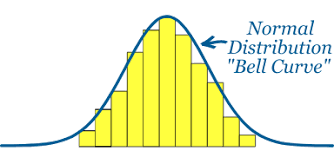
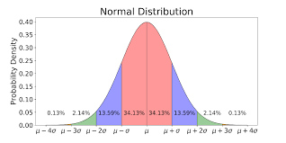
统计代写|贝叶斯分析代写Bayesian Analysis代考|The Normal Distribution
Of course, the normal density plays an important role as a model for time series. For example, as will be seen in future chapters, the normal distribution will model the observations of certain time series, such as autoregressive and moving average series. How is informative prior information expressed for the parameters $\mu$ and $\sigma$ (the mean and standard deviation)? Suppose a previous study has $m$ observations $x=\left(x_{1} x_{2}, \ldots, x_{m}\right)$, then the density of X given $\mu$ and $\sigma$ is
$$
\begin{aligned}
&f(x \mid \mu, \sigma) \propto\left[\sqrt{m} / \sqrt{2 \pi \sigma^{2}}\right] \exp -\left(m / 2 \sigma^{2}\right)(\bar{x}-\mu)^{2} \
&{\left[(2 \pi)^{-(n-1) / 2} \sigma^{-(n-1)}\right] \exp -\left(1 / 2 \sigma^{2}\right) \sum_{i=1}^{i=m}\left(x_{i}-\bar{x}\right)^{2}}
\end{aligned}
$$
This is a conjugate density for the two-parameter normal family and is called the normal-gamma density. Note it is the product of two functions, where the first, as a function of $\mu$ and $\sigma$, is the conditional density of $\mu$ given $\sigma$, with mean $\bar{x}$ and variance $\sigma^{2} / m$, while the second is a function of $\sigma$ only and is an inverse gamma density. Or equivalently, if the normal is parameterized with $\mu$ and the precision $\tau=1 / \sigma^{2}$, the conjugate distribution is as follows: (a) the conditional distribution of $\mu$ given $\tau$ is normal with mean $\bar{x}$ and precision $\mathrm{m} \tau$, and (b) the marginal distribution of $\tau$ is gamma with parameters $(m+1) / 2$ and $\sum_{i=1}^{i=m}\left(x_{i}-\bar{x}\right)^{2} / 2=(m-1) S^{2} / 2$, where $S^{2}$ is the sample variance. Thus, if one knows the results of a previous experiment, the likelihood function for $\mu$ and $\tau$ provides informative prior information for the normal population.
For example, the normal serves as the distribution of the observations of a first-order autoregressive process
$$
Y(t)=\theta Y(t-1)+W(t), t=1,2, \ldots
$$
where
$$
W(t), t=1,2, \ldots
$$
is a sequence of independent normal random variables with mean zero and precision $\tau$, and $\tau>0$. It is easy to show that the joint distribution of the $n$ observations from the AR(1) process is multivariate normal with mean vector
0 and variance covariance matrix with diagonal entries $1 / \tau\left(1-\theta^{2}\right)$ and $k$-th order covariance $\operatorname{Cov}[Y(t), Y(t+k)]=\theta^{k} / \tau\left(1-\theta^{2}\right),|\theta|<1, k=1,2, \ldots$
Note it is assumed the process is stationary, namely, $|\theta|<1$. Of course, the goal of the Bayesian analysis is to estimate the processes autoregressive parameter $\theta$ and the precision $\tau>0$. For the Bayesian analysis, a prior distribution must be assigned to $\theta$ and $\tau$, which in the conjugate prior case is a normal-gamma. The posterior analysis for the autoregressive time series results in a univariate $t$-distribution for the distribution of $\theta$ as will be shown in Chapter $5 .$
贝叶斯分析代考
统计代写|贝叶斯分析代写Bayesian Analysis代考|Bayes Theorem
贝叶斯定理基于条件概率定律:
磷[一个∣乙]=磷[乙∣一个]磷[一个]/磷[乙]
在哪里磷[一个]是 A 在知道事件结果之前发生的概率乙,磷[乙∣一个]是概率乙假设人们对事件有所了解一个, 和磷[一个∣乙]是概率一个知道那件事乙已经发生了。磷[一个]称为先验概率一个, 尽管磷[一个∣乙]称为 A 的后验概率。
贝叶斯定理的另一个版本是假设X是一个连续的可观察随机向量,并且θ∈Ω⊂R米是一个未知的参数向量,并假设条件密度X给定θ表示为F(X∣θ). 如果X=(X1,X2,…,Xn)表示大小的随机样本n来自有密度的人口F(X∣θ), 和X(θ)是先验密度θ, 那么贝叶斯定理将后验密度表示为
X(θ∣X)=C∏一世=1一世=F(X一世∣θ)X(θ),X一世∈R 和 θ∈Ω其中比例常数为C, 和项∏一世=1一世=nF(X一世∣θ)称为似然函数。密度X(θ)是先验密度θ并且表示在观察 X 之前对参数所拥有的知识。这种先验信息最有可能从其他先前的相关实验中提供给实验者。注意θ被认为是一个随机变量,并且贝叶斯定理转换了一个人的先验知识θ,由它的先验密度表示,到后验密度,并且转换是关于先验信息的组合θ用似然函数表示的样本信息。
托马斯·贝叶斯牧师的《解决机会学说中的问题的文章》1是我们主题的开始。他考虑了一个二项式实验n试验并假设概率θ成功率是均匀分布的(通过构建台球桌)并提供了一种计算方法公关(一个≤θ≤b∣X=p), 在哪里X是成功的次数n独立试验。在贝叶斯通过以下方式进行推断的意义上,这是第一次X(θ∣X), 的条件密度θ给定X. 此外,通过假设参数是均匀分布的,他假设了模糊的先验信息θ. 对参数知之甚少的先验信息类型称为非信息或模糊信息。
可以说,拉普拉斯2是最伟大的贝叶斯主义者,因为他对反概率做出了许多重大贡献(他不知道贝叶斯),从 1774 年的“Memerie sur la probabilite des Causes par la evenemens”开始,以及他自己版本的贝叶斯定理,并在一段时间内大约 40 年,最终形成了“概率分析理论”。见斯蒂格勒3和 Hald 的第 9-20 章4了解拉普拉斯对逆概率的贡献的历史。
统计代写|贝叶斯分析代写Bayesian Analysis代考|The Binomial Distribution
我们从哪里开始先验信息,这是贝叶斯定理规则的关键组成部分?贝叶斯假设参数的先验分布是均匀的,即
X(θ)=1,0≤θ≤1, 在哪里
θ是成功的常见概率n独立试验和
F(X∣θ)=(n X)θX(1−θ)n−X
在哪里X是成功的次数X=0,1,2,…,n. 对于分布X,成功的次数是二项式的,表示为X∼二项式(θ,n). 统一的先验已经使用了很多年;然而,洛斯特5提出了一个不同的先验,即
X(θ)=θ−1(1−θ)−1,0≤θ≤1
表示非信息性的信息,并且是不正确的密度函数。Lhoste 基于某些不变性原则的先验,与 Jeffreys 非常相似。6Lhoste 还推导出了标准差的非信息性先验σ有密度的正常人口
F(X∣μ,σ)=(1/2圆周率σ)经验−(1/2σ)(X−μ)2,μ∈R 和 σ>0
他使用不变性如下:他推断,先验密度σ和先验密度1/σ应该是相同的,这导致
X(σ)=1/σ
Jeffreys 的方法与为二项式和正态总体开发非信息先验的方法相似,但他也为多参数模型开发了非信息先验,包括正态密度的均值和标准差
X(μ,σ)=1/σ,μ∈R 和 σ>0
从 1920 年代到 1980 年代,非信息性先验无处不在,并包含在那个时期的所有教科书中。例如,参见 Box 和 Tiao,10泽尔纳,11和布鲁梅林。12回顾过去,具有讽刺意味的是,几乎总是使用非信息性先验信息,尽管信息性先验信息几乎总是可用的。这限制了贝叶斯方法的效用,与传统的经商方式相比,人们几乎看不到任何优势。贝叶斯方法的主要优势在于它是一种利用信息先验信息的方便、实用和合乎逻辑的方法。当然,调查人员从以前的相关研究中知道信息丰富的先验信息。
统计代写|贝叶斯分析代写Bayesian Analysis代考|The Normal Distribution
当然,正态密度作为时间序列的模型起着重要作用。例如,正如将在以后的章节中看到的,正态分布将对某些时间序列的观察进行建模,例如自回归和移动平均序列。如何为参数表达信息性先验信息μ和σ(平均值和标准差)?假设以前的研究有米观察X=(X1X2,…,X米), 那么给定 X 的密度μ和σ是
F(X∣μ,σ)∝[米/2圆周率σ2]经验−(米/2σ2)(X¯−μ)2 [(2圆周率)−(n−1)/2σ−(n−1)]经验−(1/2σ2)∑一世=1一世=米(X一世−X¯)2
这是二参数正态族的共轭密度,称为正态伽马密度。注意它是两个函数的乘积,其中第一个函数是μ和σ, 是条件密度μ给定σ, 均值X¯和方差σ2/米,而第二个是σ只有 和 是反伽马密度。或者等效地,如果法线参数化为μ和精度τ=1/σ2, 共轭分布如下: (a) 的条件分布μ给定τ均值正常X¯和精度米τ, 和 (b) 的边际分布τ是带参数的 gamma(米+1)/2和∑一世=1一世=米(X一世−X¯)2/2=(米−1)小号2/2, 在哪里小号2是样本方差。因此,如果知道先前实验的结果,则似然函数为μ和τ为正常人群提供信息丰富的先验信息。
例如,正态分布用作一阶自回归过程的观察值分布
是(吨)=θ是(吨−1)+在(吨),吨=1,2,…
在哪里
在(吨),吨=1,2,…
是一系列独立的正态随机变量,均值为 0,精度为τ, 和τ>0. 很容易证明,联合分布n来自 AR(1) 过程的观察结果是具有平均向量的多元正态分布
0 和带对角线条目的方差协方差矩阵1/τ(1−θ2)和ķ- 阶协方差这[是(吨),是(吨+ķ)]=θķ/τ(1−θ2),|θ|<1,ķ=1,2,…
请注意,假设过程是平稳的,即|θ|<1. 当然,贝叶斯分析的目标是估计过程的自回归参数θ和精度τ>0. 对于贝叶斯分析,必须将先验分布分配给θ和τ,在共轭先验情况下是正态伽马。自回归时间序列的后验分析导致单变量吨-distribution 的分布θ将在章节中展示5.

统计代写请认准statistics-lab™. statistics-lab™为您的留学生涯保驾护航。
金融工程代写
金融工程是使用数学技术来解决金融问题。金融工程使用计算机科学、统计学、经济学和应用数学领域的工具和知识来解决当前的金融问题,以及设计新的和创新的金融产品。
非参数统计代写
非参数统计指的是一种统计方法,其中不假设数据来自于由少数参数决定的规定模型;这种模型的例子包括正态分布模型和线性回归模型。
广义线性模型代考
广义线性模型(GLM)归属统计学领域,是一种应用灵活的线性回归模型。该模型允许因变量的偏差分布有除了正态分布之外的其它分布。
术语 广义线性模型(GLM)通常是指给定连续和/或分类预测因素的连续响应变量的常规线性回归模型。它包括多元线性回归,以及方差分析和方差分析(仅含固定效应)。
有限元方法代写
有限元方法(FEM)是一种流行的方法,用于数值解决工程和数学建模中出现的微分方程。典型的问题领域包括结构分析、传热、流体流动、质量运输和电磁势等传统领域。
有限元是一种通用的数值方法,用于解决两个或三个空间变量的偏微分方程(即一些边界值问题)。为了解决一个问题,有限元将一个大系统细分为更小、更简单的部分,称为有限元。这是通过在空间维度上的特定空间离散化来实现的,它是通过构建对象的网格来实现的:用于求解的数值域,它有有限数量的点。边界值问题的有限元方法表述最终导致一个代数方程组。该方法在域上对未知函数进行逼近。[1] 然后将模拟这些有限元的简单方程组合成一个更大的方程系统,以模拟整个问题。然后,有限元通过变化微积分使相关的误差函数最小化来逼近一个解决方案。
tatistics-lab作为专业的留学生服务机构,多年来已为美国、英国、加拿大、澳洲等留学热门地的学生提供专业的学术服务,包括但不限于Essay代写,Assignment代写,Dissertation代写,Report代写,小组作业代写,Proposal代写,Paper代写,Presentation代写,计算机作业代写,论文修改和润色,网课代做,exam代考等等。写作范围涵盖高中,本科,研究生等海外留学全阶段,辐射金融,经济学,会计学,审计学,管理学等全球99%专业科目。写作团队既有专业英语母语作者,也有海外名校硕博留学生,每位写作老师都拥有过硬的语言能力,专业的学科背景和学术写作经验。我们承诺100%原创,100%专业,100%准时,100%满意。
随机分析代写
随机微积分是数学的一个分支,对随机过程进行操作。它允许为随机过程的积分定义一个关于随机过程的一致的积分理论。这个领域是由日本数学家伊藤清在第二次世界大战期间创建并开始的。
时间序列分析代写
随机过程,是依赖于参数的一组随机变量的全体,参数通常是时间。 随机变量是随机现象的数量表现,其时间序列是一组按照时间发生先后顺序进行排列的数据点序列。通常一组时间序列的时间间隔为一恒定值(如1秒,5分钟,12小时,7天,1年),因此时间序列可以作为离散时间数据进行分析处理。研究时间序列数据的意义在于现实中,往往需要研究某个事物其随时间发展变化的规律。这就需要通过研究该事物过去发展的历史记录,以得到其自身发展的规律。
回归分析代写
多元回归分析渐进(Multiple Regression Analysis Asymptotics)属于计量经济学领域,主要是一种数学上的统计分析方法,可以分析复杂情况下各影响因素的数学关系,在自然科学、社会和经济学等多个领域内应用广泛。
MATLAB代写
MATLAB 是一种用于技术计算的高性能语言。它将计算、可视化和编程集成在一个易于使用的环境中,其中问题和解决方案以熟悉的数学符号表示。典型用途包括:数学和计算算法开发建模、仿真和原型制作数据分析、探索和可视化科学和工程图形应用程序开发,包括图形用户界面构建MATLAB 是一个交互式系统,其基本数据元素是一个不需要维度的数组。这使您可以解决许多技术计算问题,尤其是那些具有矩阵和向量公式的问题,而只需用 C 或 Fortran 等标量非交互式语言编写程序所需的时间的一小部分。MATLAB 名称代表矩阵实验室。MATLAB 最初的编写目的是提供对由 LINPACK 和 EISPACK 项目开发的矩阵软件的轻松访问,这两个项目共同代表了矩阵计算软件的最新技术。MATLAB 经过多年的发展,得到了许多用户的投入。在大学环境中,它是数学、工程和科学入门和高级课程的标准教学工具。在工业领域,MATLAB 是高效研究、开发和分析的首选工具。MATLAB 具有一系列称为工具箱的特定于应用程序的解决方案。对于大多数 MATLAB 用户来说非常重要,工具箱允许您学习和应用专业技术。工具箱是 MATLAB 函数(M 文件)的综合集合,可扩展 MATLAB 环境以解决特定类别的问题。可用工具箱的领域包括信号处理、控制系统、神经网络、模糊逻辑、小波、仿真等。