如果你也在 怎样代写AP统计这个学科遇到相关的难题,请随时右上角联系我们的24/7代写客服。
AP 统计主要是介绍收集、分析和从数据中得出结论的主要概念和工具。
statistics-lab™ 为您的留学生涯保驾护航 在代写AP统计方面已经树立了自己的口碑, 保证靠谱, 高质且原创的统计Statistics代写服务。我们的专家在代写AP统计方面经验极为丰富,各种代写AP统计相关的作业也就用不着说。
我们提供的AP统计及其相关学科的代写,服务范围广, 其中包括但不限于:
- Statistical Inference 统计推断
- Statistical Computing 统计计算
- Advanced Probability Theory 高等楖率论
- Advanced Mathematical Statistics 高等数理统计学
- (Generalized) Linear Models 广义线性模型
- Statistical Machine Learning 统计机器学习
- Longitudinal Data Analysis 纵向数据分析
- Foundations of Data Science 数据科学基础
统计代写|AP统计作业代写代考|Say It with Pictures
Edward R. Tufte, in his book The Visual Display of Quantitative Information, presents a number of guidelines for producing good graphics. According to the criteria, a graphical display should
- show the data:
- induce the viewer to think about the substance of the graphic rather than about the methodology, the design, the technology, or other production devices;
- avoid distorting what the data have to say.
As an example of a graph that violates some of the criteria, Tufte includes a graphic that appeared in a well-known newspaper. Figure 2-1(a), on the next page, shows a figure similar to the problem graphic, whereas part (b) of the figure shows a better rendition of the data display.
After completing this chapter, you will be able to answer the following questions.
(a) Look at the graph in Figure 2-1(a). Is it essentially a bar graph? Explain. What are some of the flaws of Figure $2-1$ (a) as a bar graph?
(b) Examine Figure 2-I(b), which shows the same information. Is it essentially a time-series graph? Explain. In what ways does the second graph seem to display the information in a clearer manner?
(See Problem 5 of the Chapter 2 Review Problems.)
统计代写|AP统计作业代写代考|Frequency Table
A task force to encourage car pooling did a study of one-way commuting distances of workers in the downtown Dallas area. A random sample of 60 of these workers was taken. The commuting distances of the workers in the sample are given in Table 2-1. Make a frequency table for these data.
SOLUTION:
(a) First decide how many classes you want. Five to 15 classes are usually used. If you use fewer than five classes, you risk losing too much information. If you use more than 15 classes, the data may not be sufficiently summarized. Let the
spread of the data and the purpose of the frequency table be your guides when selecting the number of classes. In the case of the commuting data, let’s use six classes.
(b) Next, find the class width for the six classes.
Note: To ensure that all the classes taken together cover the data, we need to increase the result of Step 1 to the next whole number, even if Step I produced a whole number. For instance, if the calculation in Step I produces the value 4 , we make the class width $5 .$
To find the class width for the commuting data, we observe that the largest distance commuted is 47 miles and the smallest is 1 mile. Using six classes, the clase width is 8 , since
Class width $=\frac{47-1}{6} \approx 7.7$ (increase to 8 )
(c) Now we determine the data range for each class.
The smallest commuting distance in our sample is 1 mile. We use this smallest data value as the lower class limit of the first class. Since the class width is 8 , we add 8 to 1 to find that the lower class limit for the second class is $9 .$ Following this pattern, we establish all the lower class limits. Then we fill in the upper class limits so that the classes span the entire range of data. Table $2-2$, on the next page, shows the upper and lower class limits for the commuting distance data.
(d) Now we are ready to tally the commuting distance data into the six classes and find the frequency for each class.
统计代写|AP统计作业代写代考|Histogram and Relative-Frequency Histogram
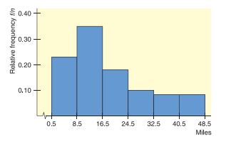
Make a histogram and a relative-frequency histogram with six bars for the data in Table 2-1 showing one-way commuting distances.
SOLUTION: The first step is to make a frequency table and a relative-frequency table with six classes. We’ll use Table $2-2$ and Table $2-3$. Figures $2-2$ and $2-3$ show the histogram and relative-frequency histogram. In both graphs, class boundaries are marked on the horizontal axis. For each class of the frequency table, make a corresponding bar with horizontal width extending from the lower boundary to the upper boundary of the respective class. For a histogram. the height of each bar is the corresponding class frequency For a relative-frequency histogram, the height of
each bar is the corresponding relative frequency. Notice that the basic shapes of the graphs are the same. The only difference involves the vertical axis. The vertical axis of the histogram shows frequencies, whereas that of the relative-frequency histogram shows relative frequencies.
Interpretation Looking at the graphs, we can observe that about half the commute distances are between 1 and 17 miles and most are less than 25 miles. It is fairly unusual for distances to exceed 40 miles or even 32 .
COMMENT The use of class boundaries in histograms assures us that the bars of the histogram touch and that no data fall on the boundaries. Both of these features are important. But a histogram displaying class boundaries may look awkward. For instance, the mileage range of $8.5$ to $16.5$ miles shown in Figure 2-2 isn’t as natural a choice as a mileage range of 8 to 16 miles. For this reason, many magazines and newspapers do not use class boundaries as labels on a histogram. Instead, some use lower class limits as labels, with the convention that a data value falling on the class limit is included in the next higher class (class to the right of the limit). Another convention is to label midpoints instead of class boundaries. Determine the default convention being used before creating frequency tables and histograms on a computer.
AP统计代写
统计代写|AP统计作业代写代考|Say It with Pictures
Edward R. Tufte 在他的《定量信息的可视化显示》一书中,提出了一些制作优质图形的指导方针。根据标准,图形显示应该
- 显示数据:
- 引导观众思考图形的实质,而不是方法、设计、技术或其他生产设备;
- 避免扭曲数据必须说明的内容。
作为违反某些标准的图表的示例,Tufte 包含了一张出现在知名报纸上的图表。下一页的图 2-1(a) 显示了与问题图形相似的图,而图的 (b) 部分显示了数据显示的更好再现。
完成本章后,您将能够回答以下问题。
(a) 看图 2-1(a)。它本质上是条形图吗?解释。图有哪些缺陷2−1(a) 作为条形图?
(b) 检查图 2-I(b),它显示了相同的信息。它本质上是一个时间序列图吗?解释。第二张图似乎以何种方式更清晰地显示了信息?
(见第 2 章复习题的第 5 题。)
统计代写|AP统计作业代写代考|Frequency Table
一个鼓励拼车的工作组对达拉斯市中心地区工人的单程通勤距离进行了研究。对其中 60 名工人进行了随机抽样。样本中工人的通勤距离见表2-1。为这些数据制作频率表。
解决方案:
(a) 首先决定你想要多少个班级。通常使用 5 到 15 个类。如果您使用的类少于五个,则可能会丢失太多信息。如果您使用超过 15 个类别,则可能无法充分汇总数据。让
数据的分布和频率表的目的是您选择类数时的指南。在通勤数据的情况下,让我们使用六个类。
(b) 接下来,找出六个类的类宽。
注意:为了确保所有的类加在一起覆盖数据,我们需要将步骤 1 的结果增加到下一个整数,即使步骤 I 产生了一个整数。例如,如果步骤 I 中的计算产生值 4 ,我们将类宽度设为5.
为了找到通勤数据的类别宽度,我们观察到最大的通勤距离是 47 英里,最小的是 1 英里。使用六个班级,班级宽度为 8 ,因为
班级宽度=47−16≈7.7(增加到 8 )
(c) 现在我们确定每个类的数据范围。
在我们的样本中,最小的通勤距离是 1 英里。我们使用这个最小的数据值作为第一类的下限。由于类宽为 8 ,我们将 8 加到 1 以发现第二类的下限为9.按照这种模式,我们建立了所有的下限。然后我们填写类上限,以便类跨越整个数据范围。桌子2−2,在下一页上,显示了通勤距离数据的上限和下限。
(d) 现在我们准备将通勤距离数据统计到六个类别中,并找到每个类别的频率。
统计代写|AP统计作业代写代考|Histogram and Relative-Frequency Histogram
为表 2-1 中的数据制作一个直方图和一个有六个条形的相对频率直方图,显示单向通勤距离。
SOLUTION: 第一步是制作一个频率表和一个六类的相对频率表。我们将使用表2−2和表2−3. 数据2−2和2−3显示直方图和相对频率直方图。在这两个图中,类边界都标记在水平轴上。对于频率表的每个类别,制作一个相应的条,其水平宽度从相应类别的下边界延伸到上边界。对于直方图。每个条的高度是相应的类频率对于相对频率直方图,高度
每个条是相应的相对频率。请注意,图形的基本形状是相同的。唯一的区别涉及垂直轴。直方图的纵轴表示频率,而相对频率直方图的纵轴表示相对频率。
解释 查看图表,我们可以观察到大约一半的通勤距离在 1 到 17 英里之间,大多数不到 25 英里。距离超过 40 英里甚至 32 英里是相当不寻常的。
评论 在直方图中使用类边界向我们保证直方图的条形接触并且没有数据落在边界上。这两个特性都很重要。但是显示类边界的直方图可能看起来很尴尬。例如,里程范围8.5到16.5图 2-2 中显示的里程不像 8 到 16 英里的里程范围那样自然。出于这个原因,许多杂志和报纸不使用类别边界作为直方图上的标签。相反,一些使用较低的类限制作为标签,约定落入类限制的数据值包含在下一个更高的类(限制右侧的类)中。另一个约定是标记中点而不是类边界。在计算机上创建频率表和直方图之前确定使用的默认约定。

Course Overview
AP Statistics is an introductory college-level statistics course that introduces students to the major concepts and tools for collecting, analyzing, and drawing conclusions from data. Students cultivate their understanding of statistics using technology, investigations, problem solving, and writing as they explore concepts like variation and distribution; patterns and uncertainty; and data-based predictions, decisions, and conclusions.
- AP Statistics Course OverviewThis resource provides a succinct description of the course and exam.PDF180.39 KB
- AP Statistics Course and Exam Description Walk-ThroughLearn more about the CED in this interactive walk-through.
- AP Statistics Course at a GlanceExcerpted from the AP Statistics Course and Exam Description, the Course at a Glance document outlines the topics and skills covered in the AP Statistics course, along with suggestions for sequencing.PDF585.66 KB
- AP Statistics Course and Exam DescriptionThis is the core document for this course. Unit guides clearly lay out the course content and skills and recommend sequencing and pacing for them throughout the year. The CED was updated in March 2021.PDF17.9 MB
- AP Statistics CED Errata SheetThis document details the updates made to the course and exam description (CED) in March 2021.PDF934.27 KB
- AP Statistics CED Scoring GuidelinesThis document details how each of the sample free-response questions in the course and exam description (CED) would be scored. This information is now in the online CED, but was not included in the binders teachers received in 2019.PDF245.87 KB
Course Content
Based on the Understanding by Design® (Wiggins and McTighe) model, this course framework provides a clear and detailed description of the course requirements necessary for student success. The framework specifies what students must know, be able to do, and understand, with a focus on three big ideas that encompass the principles and processes in the discipline of statistics. The framework also encourages instruction that prepares students for advanced coursework in statistics or other fields using statistical reasoning and for active, informed engagement with a world of data to be interpreted appropriately and applied wisely to make informed decisions.
The AP Statistics framework is organized into nine commonly taught units of study that provide one possible sequence for the course. As always, you have the flexibility to organize the course content as you like.
| Unit | Exam Weighting (Multiple-Choice Section) |
| Unit 1: Exploring One-Variable Data | 15%–23% |
| Unit 2: Exploring Two-Variable Data | 5%–7% |
| Unit 3: Collecting Data | 12%–15% |
| Unit 4: Probability, Random Variables, and Probability Distributions | 10%–20% |
| Unit 5: Sampling Distributions | 7%–12% |
| Unit 6: Inference for Categorical Data: Proportions | 12%–15% |
| Unit 7: Inference for Quantitative Data: Means | 10%–18% |
| Unit 8: Inference for Categorical Data: Chi-Square | 2%–5% |
| Unit 9: Inference for Quantitative Data: Slopes | 2%–5% |
Course Skills
The AP Statistics framework included in the course and exam description outlines distinct skills that students should practice throughout the year—skills that will help them learn to think and act like statisticians.
| Skill | Description | Exam Weighting (Multiple-Choice Section) |
| 1. Selecting Statistical Methods | Select methods for collecting and/or analyzing data for statistical inference. | 15%–23% |
| 2. Data Analysis | Describe patterns, trends, associations, and relationships in data. | 15%–23% |
| 3. Using Probability and Simulation | Explore random phenomena. | 30%–40% |
| 4. Statistical Argumentation | Develop an explanation or justify a conclusion using evidence from data, definitions, or statistical inference. | 25%–35% |
统计代写请认准statistics-lab™. statistics-lab™为您的留学生涯保驾护航。统计代写|python代写代考
随机过程代考
在概率论概念中,随机过程是随机变量的集合。 若一随机系统的样本点是随机函数,则称此函数为样本函数,这一随机系统全部样本函数的集合是一个随机过程。 实际应用中,样本函数的一般定义在时间域或者空间域。 随机过程的实例如股票和汇率的波动、语音信号、视频信号、体温的变化,随机运动如布朗运动、随机徘徊等等。
贝叶斯方法代考
贝叶斯统计概念及数据分析表示使用概率陈述回答有关未知参数的研究问题以及统计范式。后验分布包括关于参数的先验分布,和基于观测数据提供关于参数的信息似然模型。根据选择的先验分布和似然模型,后验分布可以解析或近似,例如,马尔科夫链蒙特卡罗 (MCMC) 方法之一。贝叶斯统计概念及数据分析使用后验分布来形成模型参数的各种摘要,包括点估计,如后验平均值、中位数、百分位数和称为可信区间的区间估计。此外,所有关于模型参数的统计检验都可以表示为基于估计后验分布的概率报表。
广义线性模型代考
广义线性模型(GLM)归属统计学领域,是一种应用灵活的线性回归模型。该模型允许因变量的偏差分布有除了正态分布之外的其它分布。
statistics-lab作为专业的留学生服务机构,多年来已为美国、英国、加拿大、澳洲等留学热门地的学生提供专业的学术服务,包括但不限于Essay代写,Assignment代写,Dissertation代写,Report代写,小组作业代写,Proposal代写,Paper代写,Presentation代写,计算机作业代写,论文修改和润色,网课代做,exam代考等等。写作范围涵盖高中,本科,研究生等海外留学全阶段,辐射金融,经济学,会计学,审计学,管理学等全球99%专业科目。写作团队既有专业英语母语作者,也有海外名校硕博留学生,每位写作老师都拥有过硬的语言能力,专业的学科背景和学术写作经验。我们承诺100%原创,100%专业,100%准时,100%满意。
机器学习代写
随着AI的大潮到来,Machine Learning逐渐成为一个新的学习热点。同时与传统CS相比,Machine Learning在其他领域也有着广泛的应用,因此这门学科成为不仅折磨CS专业同学的“小恶魔”,也是折磨生物、化学、统计等其他学科留学生的“大魔王”。学习Machine learning的一大绊脚石在于使用语言众多,跨学科范围广,所以学习起来尤其困难。但是不管你在学习Machine Learning时遇到任何难题,StudyGate专业导师团队都能为你轻松解决。
多元统计分析代考
基础数据: $N$ 个样本, $P$ 个变量数的单样本,组成的横列的数据表
变量定性: 分类和顺序;变量定量:数值
数学公式的角度分为: 因变量与自变量
时间序列分析代写
随机过程,是依赖于参数的一组随机变量的全体,参数通常是时间。 随机变量是随机现象的数量表现,其时间序列是一组按照时间发生先后顺序进行排列的数据点序列。通常一组时间序列的时间间隔为一恒定值(如1秒,5分钟,12小时,7天,1年),因此时间序列可以作为离散时间数据进行分析处理。研究时间序列数据的意义在于现实中,往往需要研究某个事物其随时间发展变化的规律。这就需要通过研究该事物过去发展的历史记录,以得到其自身发展的规律。
回归分析代写
多元回归分析渐进(Multiple Regression Analysis Asymptotics)属于计量经济学领域,主要是一种数学上的统计分析方法,可以分析复杂情况下各影响因素的数学关系,在自然科学、社会和经济学等多个领域内应用广泛。
MATLAB代写
MATLAB 是一种用于技术计算的高性能语言。它将计算、可视化和编程集成在一个易于使用的环境中,其中问题和解决方案以熟悉的数学符号表示。典型用途包括:数学和计算算法开发建模、仿真和原型制作数据分析、探索和可视化科学和工程图形应用程序开发,包括图形用户界面构建MATLAB 是一个交互式系统,其基本数据元素是一个不需要维度的数组。这使您可以解决许多技术计算问题,尤其是那些具有矩阵和向量公式的问题,而只需用 C 或 Fortran 等标量非交互式语言编写程序所需的时间的一小部分。MATLAB 名称代表矩阵实验室。MATLAB 最初的编写目的是提供对由 LINPACK 和 EISPACK 项目开发的矩阵软件的轻松访问,这两个项目共同代表了矩阵计算软件的最新技术。MATLAB 经过多年的发展,得到了许多用户的投入。在大学环境中,它是数学、工程和科学入门和高级课程的标准教学工具。在工业领域,MATLAB 是高效研究、开发和分析的首选工具。MATLAB 具有一系列称为工具箱的特定于应用程序的解决方案。对于大多数 MATLAB 用户来说非常重要,工具箱允许您学习和应用专业技术。工具箱是 MATLAB 函数(M 文件)的综合集合,可扩展 MATLAB 环境以解决特定类别的问题。可用工具箱的领域包括信号处理、控制系统、神经网络、模糊逻辑、小波、仿真等。