如果你也在 怎样代写金融数学Financial Mathematics这个学科遇到相关的难题,请随时右上角联系我们的24/7代写客服。
金融数学是将数学方法应用于金融问题。(有时使用的同等名称是定量金融、金融工程、数学金融和计算金融)。它借鉴了概率、统计、随机过程和经济理论的工具。传统上,投资银行、商业银行、对冲基金、保险公司、公司财务部和监管机构将金融数学的方法应用于诸如衍生证券估值、投资组合结构、风险管理和情景模拟等问题。依赖商品的行业(如能源、制造业)也使用金融数学。 定量分析为金融市场和投资过程带来了效率和严谨性,在监管方面也变得越来越重要。
statistics-lab™ 为您的留学生涯保驾护航 在代写金融数学Financial Mathematics方面已经树立了自己的口碑, 保证靠谱, 高质且原创的统计Statistics代写服务。我们的专家在代写金融数学Financial Mathematics代写方面经验极为丰富,各种代写金融数学Financial Mathematics相关的作业也就用不着说。
我们提供的金融数学Financial Mathematics及其相关学科的代写,服务范围广, 其中包括但不限于:
- Statistical Inference 统计推断
- Statistical Computing 统计计算
- Advanced Probability Theory 高等概率论
- Advanced Mathematical Statistics 高等数理统计学
- (Generalized) Linear Models 广义线性模型
- Statistical Machine Learning 统计机器学习
- Longitudinal Data Analysis 纵向数据分析
- Foundations of Data Science 数据科学基础
金融代写|金融数学代写Financial Mathematics代考|The Effective Rate of Interest
Definition: The effective rate of interest for a given period is the amount of money that one unit of principal invested at the start of a particular period will earn during that one period. It is assumed that interest is paid at the end of the period in question 2 .
If the period is one year, the effective rate of interest is also referred to as the effective annual rate of interest. This is sometimes called the APR (annual percentage rate) when expressed as a percentage. An annual effective rate of .05 would correspond to an APR of $5 \%$. As we shall see, the APR reported by various consumer credit companies is not always the same as the effective annual rate. As a result, we will use the term effective annual interest rate (or effective monthly interest rate or …) except during our discussion of the Truth in Lending Laws at the end of Chapter $6 .$
We will use the symbol $i$ for the effective rate of interest. Again, unless stated otherwise, the period is assumed to be one year. In terms of $a(t)$ we have $i=a(1)-a(0)=a(1)-1$ so we have:
Effective Rate of Interest, $i_{1}$ in period 1
$$
i_{1}=a(1)-1
$$
We can express $i$ in terms of $A(t)$ as well. Since $A(t)=P_{0} a(t)$ we have:
$$
\begin{aligned}
i_{1} &=\frac{a(1)-a(0)}{a(0)} \
&=\frac{\frac{A(1)}{P_{0}}-\frac{A(0)}{P_{0}}}{\frac{A(0)}{P_{0}}} \
&=\frac{A(1)-A(0)}{A(0)}
\end{aligned}
$$
Example 2.4: A deposit of $\$ 550$ earns $\$ 45$ in interest at the end of one year.
What is the effective annual interest rate?
Solution: We use Equation $2.7$
$$
i_{1}=\frac{A(1)-A(0)}{A(0)}=\frac{595-550}{550}=.08182
$$
This would typically be expressed as a percentage: $8.182 \%$.
金融代写|金融数学代写Financial Mathematics代考|Simple Interest
The first method of computing interest we will consider assumes that $a(t)$ is a linear function of $t$. This method is known as simple interest. It was in common use prior to the advent of calculators and computers since it is very easy to compute. It is still used in a few cases, most notably in the case of fractional time periods.
In the case of simple interest we know that $a(t)$ is a linear function and so its graph is a line. We are given two points on this line so it is easy to obtain an expression for the value of $a(t)$ at any time $t$. The slope of our line is given by
$$
\frac{(1+i)-1}{1-0}=i
$$
Since the line contains the point $(0,1)$ it’s equation is given by:
Accumulation Function for Simple Interest
$$
a(t)=1+i t
$$
In the case of simple interest, the accumulation function is a linear function with slope $i$. Figure $2.1$ is a plot of the accumulation function for the case that $i=.05$ :The amount function is just as easy to compute:
Amount Function for Simple Interest
$$
A(t)=F V=P V \cdot(1+i t)
$$
This is a line with y-intercept $=P V$ and slope $=P V_{i}$.
金融代写|金融数学代写Financial Mathematics代考|Compound Interest
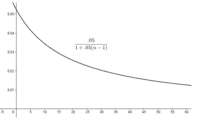
Simple interest computes the interest in each period based solely on the amount of the initial deposit. If there are no withdrawals during the life of the transaction, the amount on deposit increases over time while the amount of interest paid at the end of each period remains constant. As we just saw this results in a declining effective rate of interest when we use simple interest. If $\$ 400$ is deposited at $5 \%$ simple interest the amount on deposit after three years is $\$ 460$. However (using simple interest) the interest paid at the end of year 4 is still only $\$ 20$ (5\% of $\$ 400)$. If interest was paid based on the amount on deposit at the end of year 3 , the interest at the end of year 4 would be $(.05) \cdot \$ 460=\$ 23$
When the interest paid at the end of a given period is based on the accumulated value of the principal at the start of that period rather than on the amount of the original deposit we obtain what is known as compound interest.
To find the formula for the accumulation function in the case of compound interest, we compute the earned interest at the end of each period, add this to the previous balance, and use that number as the principal in computing the interest for the next period. See Table 2.1.
This leads us to believe that the following formula holds for the accumulation function in the case of compound interest
Accumulation Function: Compound Interest
$$
a(n)=(1+i)^{n}
$$
You can prove Equation $2.13$ for whole numbers using mathematical induction. We have calculated this result using only integral values for the time on deposit. If interest is only paid at integral multiples of the period, $a(n)$ is a step function:
$$
a(n)= \begin{cases}1 & 0 \leq n<1 \ 1+i & 1 \leq n<2 \ (1+i)^{2} & 2 \leq n<3 \ (1+i)^{3} & 3 \leq n<4 \ \text { etc.. } & \end{cases}
$$
If we assume that interest can be collected at any time in the life of the investment, it’s natural to extend this step function to include real $t \geq 0$. We thus obtain the function $a(t)=(1+i)^{t}$ defined for all real numbers $t$ which is the continuous, differentiable extension of Equation $2.3$
Accmulation Function for Compound Interest
$$
a(t)=(1+i)^{t}
$$

金融数学代考
金融代写|金融数学代写Financial Mathematics代考|The Effective Rate of Interest
定义:给定时期的有效利率是在特定时期开始时投资的一单位本金在该时期内将赚取的金额。假设利息在问题 2 的期末支付。
如果期限为一年,则实际利率也称为实际年利率。当以百分比表示时,这有时称为 APR(年度百分比率)。0.05 的年有效利率相当于 APR5%. 正如我们将看到的,各个消费信贷公司报告的 APR 并不总是与实际年利率相同。因此,我们将使用术语有效年利率(或有效月利率或……),除非我们在本章末尾讨论贷款法的真相6.
我们将使用符号一世为有效利率。同样,除非另有说明,否则该期限假定为一年。按照一个(吨)我们有一世=一个(1)−一个(0)=一个(1)−1所以我们有:
有效利率,一世1在第 1 期
一世1=一个(1)−1
我们可以表达一世按照一个(吨)也是。自从一个(吨)=磷0一个(吨)我们有:
一世1=一个(1)−一个(0)一个(0) =一个(1)磷0−一个(0)磷0一个(0)磷0 =一个(1)−一个(0)一个(0)
例 2.4:存款$550赚$45一年结束时的利息。
什么是有效年利率?
解决方案:我们使用方程式2.7
一世1=一个(1)−一个(0)一个(0)=595−550550=.08182
这通常表示为百分比:8.182%.
金融代写|金融数学代写Financial Mathematics代考|Simple Interest
我们将考虑的第一种计算兴趣的方法假设一个(吨)是一个线性函数吨. 这种方法被称为单利。它在计算器和计算机出现之前就已经普遍使用,因为它很容易计算。它仍然在少数情况下使用,尤其是在分数时间段的情况下。
在简单兴趣的情况下,我们知道一个(吨)是一个线性函数,所以它的图形是一条线。我们在这条线上有两个点,因此很容易获得值的表达式一个(吨)随时吨. 我们线的斜率由下式给出
(1+一世)−11−0=一世
由于该线包含该点(0,1)它的方程由下式给出:
单利的累积函数
一个(吨)=1+一世吨
在简单的情况下,累积函数是具有斜率的线性函数一世. 数字2.1是累积函数的图一世=.05:金额函数同样容易计算:
Amount Function for Simple Interest
一个(吨)=F在=磷在⋅(1+一世吨)
这是一条带有 y 截距的线=磷在和坡度=磷在一世.
金融代写|金融数学代写Financial Mathematics代考|Compound Interest
单利仅根据初始存款金额计算每个期间的利息。如果在交易期间没有提款,存款金额会随着时间的推移而增加,而在每个期间结束时支付的利息金额保持不变。正如我们刚刚看到的,当我们使用单利时,这会导致有效利率下降。如果$400存放在5%单利 三年后的存款金额为$460. 但是(使用单利)在第 4 年末支付的利息仍然只有$20(5\% 的$400). 如果按第 3 年末的存款金额支付利息,则第 4 年末的利息为(.05)⋅$460=$23
当在给定期间结束时支付的利息基于该期间开始时本金的累积值而不是原始存款金额时,我们获得了所谓的复利。
为了在复利的情况下找到累积函数的公式,我们计算每个期末赚取的利息,将其添加到上一个余额中,并使用该数字作为计算下一期利息的本金。见表 2.1。
这使我们相信,在复利累积函数的情况下,以下公式适用于
累积函数: 复利
一个(n)=(1+一世)n
你可以证明方程2.13使用数学归纳法计算整数。我们仅使用存款时间的整数值计算了此结果。如果利息只支付期间的整数倍,一个(n)是阶跃函数:
一个(n)={10≤n<1 1+一世1≤n<2 (1+一世)22≤n<3 (1+一世)33≤n<4 ETC..
如果我们假设可以在投资生命周期的任何时间收取利息,那么很自然地扩展这个阶梯函数以包括真实的吨≥0. 因此我们得到函数一个(吨)=(1+一世)吨为所有实数定义吨这是方程的连续、可微扩展2.3
复利累积函数
一个(吨)=(1+一世)吨

统计代写请认准statistics-lab™. statistics-lab™为您的留学生涯保驾护航。
金融工程代写
金融工程是使用数学技术来解决金融问题。金融工程使用计算机科学、统计学、经济学和应用数学领域的工具和知识来解决当前的金融问题,以及设计新的和创新的金融产品。
非参数统计代写
非参数统计指的是一种统计方法,其中不假设数据来自于由少数参数决定的规定模型;这种模型的例子包括正态分布模型和线性回归模型。
广义线性模型代考
广义线性模型(GLM)归属统计学领域,是一种应用灵活的线性回归模型。该模型允许因变量的偏差分布有除了正态分布之外的其它分布。
术语 广义线性模型(GLM)通常是指给定连续和/或分类预测因素的连续响应变量的常规线性回归模型。它包括多元线性回归,以及方差分析和方差分析(仅含固定效应)。
有限元方法代写
有限元方法(FEM)是一种流行的方法,用于数值解决工程和数学建模中出现的微分方程。典型的问题领域包括结构分析、传热、流体流动、质量运输和电磁势等传统领域。
有限元是一种通用的数值方法,用于解决两个或三个空间变量的偏微分方程(即一些边界值问题)。为了解决一个问题,有限元将一个大系统细分为更小、更简单的部分,称为有限元。这是通过在空间维度上的特定空间离散化来实现的,它是通过构建对象的网格来实现的:用于求解的数值域,它有有限数量的点。边界值问题的有限元方法表述最终导致一个代数方程组。该方法在域上对未知函数进行逼近。[1] 然后将模拟这些有限元的简单方程组合成一个更大的方程系统,以模拟整个问题。然后,有限元通过变化微积分使相关的误差函数最小化来逼近一个解决方案。
tatistics-lab作为专业的留学生服务机构,多年来已为美国、英国、加拿大、澳洲等留学热门地的学生提供专业的学术服务,包括但不限于Essay代写,Assignment代写,Dissertation代写,Report代写,小组作业代写,Proposal代写,Paper代写,Presentation代写,计算机作业代写,论文修改和润色,网课代做,exam代考等等。写作范围涵盖高中,本科,研究生等海外留学全阶段,辐射金融,经济学,会计学,审计学,管理学等全球99%专业科目。写作团队既有专业英语母语作者,也有海外名校硕博留学生,每位写作老师都拥有过硬的语言能力,专业的学科背景和学术写作经验。我们承诺100%原创,100%专业,100%准时,100%满意。
随机分析代写
随机微积分是数学的一个分支,对随机过程进行操作。它允许为随机过程的积分定义一个关于随机过程的一致的积分理论。这个领域是由日本数学家伊藤清在第二次世界大战期间创建并开始的。
时间序列分析代写
随机过程,是依赖于参数的一组随机变量的全体,参数通常是时间。 随机变量是随机现象的数量表现,其时间序列是一组按照时间发生先后顺序进行排列的数据点序列。通常一组时间序列的时间间隔为一恒定值(如1秒,5分钟,12小时,7天,1年),因此时间序列可以作为离散时间数据进行分析处理。研究时间序列数据的意义在于现实中,往往需要研究某个事物其随时间发展变化的规律。这就需要通过研究该事物过去发展的历史记录,以得到其自身发展的规律。
回归分析代写
多元回归分析渐进(Multiple Regression Analysis Asymptotics)属于计量经济学领域,主要是一种数学上的统计分析方法,可以分析复杂情况下各影响因素的数学关系,在自然科学、社会和经济学等多个领域内应用广泛。
MATLAB代写
MATLAB 是一种用于技术计算的高性能语言。它将计算、可视化和编程集成在一个易于使用的环境中,其中问题和解决方案以熟悉的数学符号表示。典型用途包括:数学和计算算法开发建模、仿真和原型制作数据分析、探索和可视化科学和工程图形应用程序开发,包括图形用户界面构建MATLAB 是一个交互式系统,其基本数据元素是一个不需要维度的数组。这使您可以解决许多技术计算问题,尤其是那些具有矩阵和向量公式的问题,而只需用 C 或 Fortran 等标量非交互式语言编写程序所需的时间的一小部分。MATLAB 名称代表矩阵实验室。MATLAB 最初的编写目的是提供对由 LINPACK 和 EISPACK 项目开发的矩阵软件的轻松访问,这两个项目共同代表了矩阵计算软件的最新技术。MATLAB 经过多年的发展,得到了许多用户的投入。在大学环境中,它是数学、工程和科学入门和高级课程的标准教学工具。在工业领域,MATLAB 是高效研究、开发和分析的首选工具。MATLAB 具有一系列称为工具箱的特定于应用程序的解决方案。对于大多数 MATLAB 用户来说非常重要,工具箱允许您学习和应用专业技术。工具箱是 MATLAB 函数(M 文件)的综合集合,可扩展 MATLAB 环境以解决特定类别的问题。可用工具箱的领域包括信号处理、控制系统、神经网络、模糊逻辑、小波、仿真等。