统计代写|数据结构作业代写data structure代考|Divide and Conquer Master Theorem
如果你也在 怎样代写数据结构data structure这个学科遇到相关的难题,请随时右上角联系我们的24/7代写客服。
数据结构是一种用于存储和组织数据的存储。它是一种在计算机上安排数据的方式,以便可以有效地访问和更新。根据你的要求和项目,为你的项目选择正确的数据结构很重要。
statistics-lab™ 为您的留学生涯保驾护航 在代写数据结构data structure方面已经树立了自己的口碑, 保证靠谱, 高质且原创的统计Statistics代写服务。我们的专家在代写数据结构data structure方面经验极为丰富,各种代写数据结构data structure相关的作业也就用不着说。
我们提供的数据结构data structure及其相关学科的代写,服务范围广, 其中包括但不限于:
- Statistical Inference 统计推断
- Statistical Computing 统计计算
- Advanced Probability Theory 高等楖率论
- Advanced Mathematical Statistics 高等数理统计学
- (Generalized) Linear Models 广义线性模型
- Statistical Machine Learning 统计机器学习
- Longitudinal Data Analysis 纵向数据分析
- Foundations of Data Science 数据科学基础
统计代写|数据结构作业代写data structure代考|Problems & Solutions
For each of the following recurrences, give an expression for the runtime $T(n)$ if the recurrence can be solved with the Master Theorem. Otherwise, indicate that the Master Theorem does not apply.
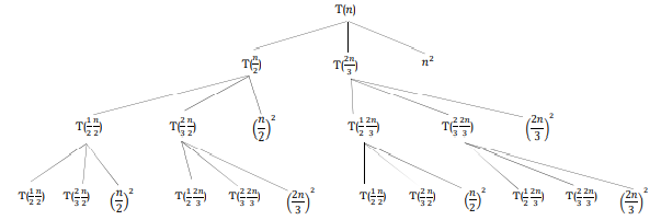
Problem-1 $T(n)=3 T(n / 2)+n^{2}$
Solutions $T(n)=3 T(n / 2)+n^{2} \Rightarrow T(n)=\Theta\left(n^{2}\right)$ (Mnster Theorem Case 3.a)
Problem-2 $T(n)=4 T(n / 2)+n^{2}$
Solution: $T(n)=4 T(n / 2)+n^{2}=>T(n)=\theta\left(n^{2} \log n\right)$ (Master Theorem Case 2.a)
Problem-3 $T(n)=T(n / 2)+n^{2}$
Solution: $T(n)=T(n / 2)+n^{2}=>\theta\left(n^{2}\right)$ (Master Theorcm Casc 3.a)
Problem-4 $T(n)=2^{n} T(n / 2)+n^{n}$
Solution: $T(n)=2^{n} T(n / 2)+n^{n} \rightarrow$ Does not apply $(a$ is not constant)
Problems $T(n)=16 T(n / 4)+n$
Solution: $T(n)=16 T(n / 4)+n=T(n)=\Theta\left(n^{2}\right)$ (Master Theorem Case 1)
Problem-6 $T(n)=2 T(n / 2)+n \log n$
Solution: $T(n)=2 T(n / 2)+n \log n=>T(n)=\theta\left(n \log ^{2} n\right)$ (Master Theorem Case 2.a)
Problem-7 $T(n)=2 T(n / 2)+n / \log n$
Solution: $T(n)=2 T(n / 2)+n / \log n=>T(n)=\theta($ nloglog$n)$ (Master Theorem Case 2.b)
Problem-8 $T(n)=2 T(n / 4)+n^{0.51}$
Solution: $T(n)=2 T(n / 4)+n^{0.51}=>T(n)=\theta\left(n^{0.51}\right)$ (Mnster Theorcm Casc 3.b)
Problem-9 $T(n)=0.5 T(n / 2)+1 / n$
Solution: $T(n)=0.5 T(n / 2)+1 / n=>$ Does not apply $(a<1)$ Problem-10 $T(n)=6 T(n / 3)+n^{2} \log n$ Solution: $T(n)=6 T(n / 3)+n^{2} \log n=>T(n)=\Theta\left(n^{2} \log n\right)$ (Master Theorem Case 3.a)
Problem-11 $T(n)=64 T(n / 8)-n^{2} \log n$
Solution: $T(n)=64 T(n / 8)-n^{2} \log n=>$ Does not apply (function is not positive)
Problem-12 $T(n)=7 T(n / 3)+n^{2}$
Solution: $T(n)=7 T(n / 3)+n^{2}=>T(n)=\Theta\left(n^{2}\right)$ (Master Theorem Case 3.as)
Problem-18 $T(n)=4 T(n / 2)+\log n$
Solution: $T(n)=4 T(n / 2)+\log n=T(n)=\theta\left(n^{2}\right)$ (Master Theorem Case 1)
Problem-14 $T(n)=16 T(n / 4)+n !$
Solution: $T(n)=16 T(n / 4)+n ! \Rightarrow T(n)=\Theta(n !)$ (Master Theorem Case 3.a)
Problem-15 $T(n)=\sqrt{2} T(n / 2)+\log n$
Solution: $T(n)=\sqrt{2} T(n / 2)+\log n=>T(n)=\Theta(\sqrt{n})$ (Master Theorem Case 1)
Problem-16 $T(n)=3 T(n / 2)+n$
Solution: $T(n)=3 T(n / 2)+n=>T(n)=\Theta\left(n^{\log 3}\right)$ (Master Theorem Case 1)
Problem-17 $T(n)=3 T(n / 3)+\sqrt{n}$
Solutiont $T(n)=3 T(n / 3)+\sqrt{n} \Rightarrow T(n)=\Theta(n)$ (Master Theorem Case 1)
Problem-18 $T(n)=4 T(n / 2)+c n$
Solution: $T(n)=4 T(n / 2)+c n=T(n)=\Theta\left(n^{2}\right)$ (Master Theorem Case 1)
Problem-19 $\bar{T}(n)=3 \bar{T}(n / 4)+n \log n$
Solution: $T(n)=3 T(n / 4)+n \log n=>T(n)=\Theta(n \log n)$ (Master Theorem Case 3.a)
Problem-20 $T(n)=3 T(n / 3)+n / 2$
Solution: $T(n)=3 T(n / 3)+n / 2=>T(n)=\Theta(n \log n)$ (Master Theorem Case 2.a)
统计代写|数据结构作业代写data structure代考|Method of Guessing and Confirming
Now, let us discuss a method which can be used to solve any recurrence. The basic idea behaind this method is:
guess the answer; and then prove it correct by induction.
In other words, it addresses the question: What if the given recurrence doesn’t seem to match with any of these inaster theoreml methods? If we guess a solution and then try to verify our guess inductively, usually either the proof will succeed (in which case we are done), or the proof will fail (in which case the failure will help us refine our guess).
As iul cximule, comsides toe rexuncue T(n) $-\sqrt{n} T(\sqrt{n})+\mathrm{~ t . ~ T h i s ~ d o}$ observing the recurrence gives us the impression that it is similar to the divide and conquer method (dividing the problem into $\sqrt{n}$ subproblems each with size $\sqrt{n})$. As we can see, the size of the subproblems at the first level of recursion is $n$. So, let us guess that T(n) – O(nlogn), and then try to prowe that our guess is correct.
Let’s start by trying to prove an upper bound T $(n) \leq$ cnlogn:
$$
\begin{aligned}
T(n) &=\sqrt{n} T(\sqrt{n})+n \
& \leq \sqrt{n} \cdot c \sqrt{n} \log \sqrt{n}+n \
&=n \cdot c \log \sqrt{n}+n \
&=n \cdot c \cdot \frac{1}{2} \cdot \log n+n \
& \leq c n \log n
\end{aligned}
$$
The last inequality assumes only that $1 \leq c, \frac{1}{2}$. $\log n$. This is correct if $n$ is sufficicntly lange and for aary constant $c$, no maatter how small. From the abowe proof, we can see that our guess is correct for the upper bound. Now, let us prone the lower bound for this recurrence.
统计代写|数据结构作业代写data structure代考|Amortized Analysis
Amortized analysis refers to deternaining the time-iveraged runaing time for a sequence of operations. It is differeat froma average case analysis, because amortized analysis does not make any assmption about the distribution of the data values, whereas average case analysis assumes the data are not “bad” (c.g., sone sorting algonthms do well on average oxer all input orderangs but very badly on certain input orderings). That is, anbortized analysis is a worst-case analysis, but for a sequence of operations rather than for individual operations.
The nootination for anortizcd anahsis is to better undersiand the nunning tinve of certain techniqucs, where standard worstecase analysis provides an overly pessimistic bouad. Amortized analysas generally applies to a method that consists of a sequence of operations, where the vast majority of the operations are cheap, but some of the operations are expeasive. If we can show that the expensive operations are particularly rare, we can change them to the cheap operations, and only bound the cheap operations.
The general approach is to assign an autificial cost to each operation in the sequence, such that the total of the artificial costs for the sequence of operations bounds the total of the real costs for the scquence. Thas iutificial cost is called the anortized cost of an operation. To analyze the rumning time, the amortized cost thus is a correct way of understanding the overall ruming time – but uote that particular operations can still take louger so it is not a way of bounding the nuning time of any individual operation in the sequence.
Whes one event in a sequence affects the cost of later events:
- Oae particular task nay be expensive.
- But it may leave data structure in a state that the next few operations become easier.
Dermple: Let us consider an array of elenucuts from which we wat to find the $k^{\text {th }}$ smallest elenaent. We can solve this problem using sorting. After sorting the given array, we just need to retura the $k^{\text {th }}$ clement fron it. The cost of performing the sort (assunuing conparison-based sorting algorithm) is $\mathrm{O}\left(n \log n\right.$. If we perform $n$ such selections then the average cost of each selection is $\mathrm{O}(\mathrm{nlog} / \mathrm{n})=\mathrm{O}(\log )^{\mathrm{l}}$. This clearly indicates that sorting ouce is roducing the conplexity of subsequcat operations.
数据结构代写
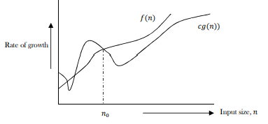
统计代写|数据结构作业代写data structure代考|Omega-Ω Notation
类似于这讨论,这个符号给出了给定算法的更严格的下限,我们将其表示为F(n)=Ω(G(n)). 那 nueans,在较大的值n,更紧的下界F(n)是G(n). 这Ω符号可以定义为\Omega(g(n))={f(n)$ 存在正常数 $\mathrm{c}$ 和 $n_{0}$ 使得 $0 \leq c g(n) \leq f(n)$ 为所有 $\left.\mathrm{n} \geq n_{0}\right} \cdot g(n)\Omega(g(n))={f(n)$ 存在正常数 $\mathrm{c}$ 和 $n_{0}$ 使得 $0 \leq c g(n) \leq f(n)$ 为所有 $\left.\mathrm{n} \geq n_{0}\right} \cdot g(n)是一个渐近紧下界F(n). 我们的目标是提供最大的增长率G(n)小于或等于给定算法的增长率F(n).
例如,如果F(n)−100n3+10n+50,G(n)是Ω(n2).
Ω示例
Exrmple-1 查找下限F(n)=5n2.
解决方案∃C,n0这样:0≤Cn2≤5n2⇒Cn2≤5n2⇒C=5和n0=1 ∴5n2=Ω(n2)和C=5和n0−1
Eample-2 证明F(n)=100n+5≠Ω(n2).
解决方案∃C,n0这样:0≤Cn22≤100n+5
100n+5≤100n+5n(∀n≥1)=105n Cn2≤105n⇒n(Cn−105)≤0
自从n是积极的⇒Cn−105≤0⇒n≤105/C
⇒矛盾:n不能小于常数
Example-32n=Ω(n),n2=Ω(n2),日志n=Ω(日志n).
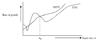
统计代写|数据结构作业代写data structure代考|Theta- Notation
此符号决定给定函数(算法)的上限和下限是否相同。算法的平均 ruming time 介于下限和上限之间。如果上界 (O) 和下界 (S2) 给出相同的结果,则θ符号墙也有保存速度的增长。一种举个例子,让我们假设F(n)=10n+n是表达式。然后,它的紧上界G(n)是这(n). 最好情况下的增长率是G(n)=这(n).
在这种情况下,最好情况和最坏情况下的增长率是相同的。结果,平均情况也将相同。对于给定的函数(算法),如果增长率(边界)为这和Ω不一样,那么增长率为θcnse 可能不一样。在这种情况下,我们需要考虑所有可能的 tinve 复杂性并计算它们的平均值(例如,对于一个快速的 sont itrerige 案例,请参阅 Sorting chapuca)。
现在考虑一下θ意志。它被定义为θ(G(n))=FF(n): 存在正常数C1, C2和n0使得 0 sC1G(n)⩽F(n)⩽C2G(n)对全部n≈n0]⋅G(n)是一个等距紧的botmdF(n). θ(G(n))是具有增长 a 的语义顺序的函数集G(n).
θ示例
示例 1 查找θ开往F(n)=n22−n2
解决方案:n25≤n22=n2≤n2, 对全部,n≥2
∴n22−n2=θ(n2)和C1=1/5,C2=1和n0=2
Ermple 2 证明n≠θ(n2)
解决方案:C1n2≤n≤C2n2⇒仅适用于:n≤1/C1
∴n≠θ(n2)
2ramp 8 证明6n3−θ(n2)
解决方案:C1n2≤6n3≤C2n2⇒仅适用于:n≤C2/6
∴6n3≠θ(n2)
Jrample 4 证明n≠θ(日志n)
解决方案:C1日志n≤n≤C7日志n⇒C7≥n 安静的 ⋅∀n≥nn– 不可能的
重要说明
对于分析(最佳情况、最坏情况和平均值),我们尝试给出上限 (O) 和下限 (S2) 以及平均 rumáng 时间 (θ)。从上面的例子中,还应该清楚的是,对于给定的函数(algonthm),得到上界(O)和下界(S2)和平均数(θ)不总是可能的。例如,如果我们正在讨论算法的最佳情况,我们会尝试给出上限(这)和下限(Ω)和平均运行时间(θ).
在更新的章节中,我们通常关注上界 (O),因为知道算法的下界 (S2) 没有实际意义,我们使用θ符号如果上boumd(这)和下限(Ω)是相同的。
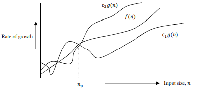
统计代写|数据结构作业代写data structure代考|Master Theorem for Divide and Conquer Recurrences
所有分治算法(也在分治一章中详细讨论)将问题划分为子问题,其中的缓存是原始问题的一部分,然后执行额外的工作来计算最终答案。举个例子,一个归并排序算法[详情请参考排序章节]对两个子问题进行运算,其中的cach的大小是原来的一半,然后执行这(n)合并的额外工作。这给出了运行时间方程:
吨(n)=2吨(n2)+这(n)
以下定理可用于确定分治算法的运行时间。对于给定的程序(算法),首先我们尝试找到问题的递归关系。如果递归是下面的形式,那么我们可以直接给出答案而不用完全解决它。如果重复是形式吨(n)=一种吨(nb)+θ(nķ日志pn), 在哪里一种≥1,b>1,ķ≥0和p是实数,则:
1) 如果一种>bķ, 然后吨(n)=θ(n日志Gb)
2) 如果一种=bķ
一种。如果p>−1, 然后吨(n)=θ(n日志b一种日志p+1n)湾。如果p=−1, 然后吨(n)=θ(n日志l日志日志n)C。如果p<−1, 然后吨(n)=θ(n日志b一种)
3) 如果一种<bķ
一种。如果p≥0, 然后吨(n)=θ(nķ日志pn)
湾。如果p<0, 然后吨(n)=这(nķ)

统计代写请认准statistics-lab™. statistics-lab™为您的留学生涯保驾护航。统计代写|python代写代考
随机过程代考
在概率论概念中,随机过程是随机变量的集合。 若一随机系统的样本点是随机函数,则称此函数为样本函数,这一随机系统全部样本函数的集合是一个随机过程。 实际应用中,样本函数的一般定义在时间域或者空间域。 随机过程的实例如股票和汇率的波动、语音信号、视频信号、体温的变化,随机运动如布朗运动、随机徘徊等等。
贝叶斯方法代考
贝叶斯统计概念及数据分析表示使用概率陈述回答有关未知参数的研究问题以及统计范式。后验分布包括关于参数的先验分布,和基于观测数据提供关于参数的信息似然模型。根据选择的先验分布和似然模型,后验分布可以解析或近似,例如,马尔科夫链蒙特卡罗 (MCMC) 方法之一。贝叶斯统计概念及数据分析使用后验分布来形成模型参数的各种摘要,包括点估计,如后验平均值、中位数、百分位数和称为可信区间的区间估计。此外,所有关于模型参数的统计检验都可以表示为基于估计后验分布的概率报表。
广义线性模型代考
广义线性模型(GLM)归属统计学领域,是一种应用灵活的线性回归模型。该模型允许因变量的偏差分布有除了正态分布之外的其它分布。
statistics-lab作为专业的留学生服务机构,多年来已为美国、英国、加拿大、澳洲等留学热门地的学生提供专业的学术服务,包括但不限于Essay代写,Assignment代写,Dissertation代写,Report代写,小组作业代写,Proposal代写,Paper代写,Presentation代写,计算机作业代写,论文修改和润色,网课代做,exam代考等等。写作范围涵盖高中,本科,研究生等海外留学全阶段,辐射金融,经济学,会计学,审计学,管理学等全球99%专业科目。写作团队既有专业英语母语作者,也有海外名校硕博留学生,每位写作老师都拥有过硬的语言能力,专业的学科背景和学术写作经验。我们承诺100%原创,100%专业,100%准时,100%满意。
机器学习代写
随着AI的大潮到来,Machine Learning逐渐成为一个新的学习热点。同时与传统CS相比,Machine Learning在其他领域也有着广泛的应用,因此这门学科成为不仅折磨CS专业同学的“小恶魔”,也是折磨生物、化学、统计等其他学科留学生的“大魔王”。学习Machine learning的一大绊脚石在于使用语言众多,跨学科范围广,所以学习起来尤其困难。但是不管你在学习Machine Learning时遇到任何难题,StudyGate专业导师团队都能为你轻松解决。
多元统计分析代考
基础数据: $N$ 个样本, $P$ 个变量数的单样本,组成的横列的数据表
变量定性: 分类和顺序;变量定量:数值
数学公式的角度分为: 因变量与自变量
时间序列分析代写
随机过程,是依赖于参数的一组随机变量的全体,参数通常是时间。 随机变量是随机现象的数量表现,其时间序列是一组按照时间发生先后顺序进行排列的数据点序列。通常一组时间序列的时间间隔为一恒定值(如1秒,5分钟,12小时,7天,1年),因此时间序列可以作为离散时间数据进行分析处理。研究时间序列数据的意义在于现实中,往往需要研究某个事物其随时间发展变化的规律。这就需要通过研究该事物过去发展的历史记录,以得到其自身发展的规律。
回归分析代写
多元回归分析渐进(Multiple Regression Analysis Asymptotics)属于计量经济学领域,主要是一种数学上的统计分析方法,可以分析复杂情况下各影响因素的数学关系,在自然科学、社会和经济学等多个领域内应用广泛。
MATLAB代写
MATLAB 是一种用于技术计算的高性能语言。它将计算、可视化和编程集成在一个易于使用的环境中,其中问题和解决方案以熟悉的数学符号表示。典型用途包括:数学和计算算法开发建模、仿真和原型制作数据分析、探索和可视化科学和工程图形应用程序开发,包括图形用户界面构建MATLAB 是一个交互式系统,其基本数据元素是一个不需要维度的数组。这使您可以解决许多技术计算问题,尤其是那些具有矩阵和向量公式的问题,而只需用 C 或 Fortran 等标量非交互式语言编写程序所需的时间的一小部分。MATLAB 名称代表矩阵实验室。MATLAB 最初的编写目的是提供对由 LINPACK 和 EISPACK 项目开发的矩阵软件的轻松访问,这两个项目共同代表了矩阵计算软件的最新技术。MATLAB 经过多年的发展,得到了许多用户的投入。在大学环境中,它是数学、工程和科学入门和高级课程的标准教学工具。在工业领域,MATLAB 是高效研究、开发和分析的首选工具。MATLAB 具有一系列称为工具箱的特定于应用程序的解决方案。对于大多数 MATLAB 用户来说非常重要,工具箱允许您学习和应用专业技术。工具箱是 MATLAB 函数(M 文件)的综合集合,可扩展 MATLAB 环境以解决特定类别的问题。可用工具箱的领域包括信号处理、控制系统、神经网络、模糊逻辑、小波、仿真等。