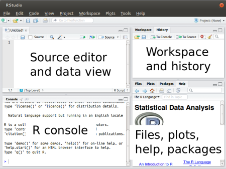
统计代写|R 统计计算作业代写Introduction to Statistical Computing with R代考|Interactive plotting
如果你也在 怎样代写R 统计计算Introduction to Statistical Computing with R这个学科遇到相关的难题,请随时右上角联系我们的24/7代写客服。
R 统计计算和统计计算是采用计算、图形和数字方法解决统计问题的两个领域,这使得多功能的R语言成为这些领域的理想计算环境。
statistics-lab™ 为您的留学生涯保驾护航 在代写R 统计计算Introduction to Statistical Computing with R方面已经树立了自己的口碑, 保证靠谱, 高质且原创的统计Statistics代写服务。我们的专家在代写R 统计计算方面经验极为丰富,各种代写R 统计计算Introduction to Statistical Computing with R相关的作业也就用不着说。
我们提供的R 统计计算Introduction to Statistical Computing with R代写及其相关学科的代写,服务范围广, 其中包括但不限于:
- Statistical Inference 统计推断
- Statistical Computing 统计计算
- Advanced Probability Theory 高等楖率论
- Advanced Mathematical Statistics 高等数理统计学
- (Generalized) Linear Models 广义线性模型
- Statistical Machine Learning 统计机器学习
- Longitudinal Data Analysis 纵向数据分析
- Foundations of Data Science 数据科学基础
统计代写|R 统计计算作业代写Introduction to Statistical Computing with R代考|The manipulate function
The most important tunction of the manipulale package is manipulale. The value of the first argument of the manipulate function must be an expression or function that generates a plot. Various arguments can be added to define custom sliders, buttons, checkboxes, or pickers (drop-down menus) that are to be used in a small user interface (a manipulator) to manipulate a graphic. The following is an example of a manipulator:If these statements are executed, a plot is created with a gearbox icon at the top left-hand side. Clicking on the icon opens a small menu box with a checkbox, a slider, and a button. Each time you move the slider or click on a button or checkbox, the variables (pch, cex, and axes) are set to the value chosen in the menu, and the plot is recreated.
统计代写|R 统计计算作业代写Introduction to Statistical Computing with R代考|Using more options of manipulate
After a manipulator is launched it creates the plot with initial values and waits for an action of the user. When one of the controls is altered, the following actions are performed:
- The values returned by the controls are substituted in the corresponding variables
- The expression in the first argument is re-evaluated, causing a new plot
The expression in the first argument need not be a single expression. In fact, the firs argument can be a sequence of complex expressions enclosed by curly braces {} . Inside those braces you may use any $\mathrm{R}$ command, either plotting or otherwise.
If executing one of the commands takes a long time, for example because it involves computing a complex model, you may store the results for retrieval on reruns after the user controls using manipulatorsetstate and manipulatorGetstate.
In the if statement of the first line, we check whether the variable model was stored before. If it wasn’t, manipulatorGet State returns NULL. If the variable was not stored before, it is computed with $1 \mathrm{~m}$ and stored using manipulatorsetstate, here under the name model. This branch is executed only the first time the expression is evaluated. We’ve added a print command, so the difference between calls will be clearly noticed. If the variable has been stored before (after the first evaluation), it is retrieved using manipulatorGetState in the else branch. Finally, a plot of original versus predicted values is made. The manipulator allows for choosing the color of points.
There is one more function specific to manipulate, which can be used in the set of expressions passed to manipulate, namely manipulatorMouseclick. This function returns NULL when a plot was made because a menu item was changed, otherwise it returns a list of plotting coordinates in several coordinate systems.
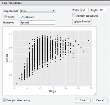
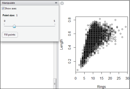
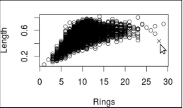
Here is an example where we plot Length against the number of Rings in the abalone dataset and use the mouse to plot an extra cross:
manipulate ( {
plot (Length Rings, data=abalone)
xy <- manipulatorMouseclick()
if $(1$ is.null $(x y))$ points (xy\$user $x$, xy\$usery, pch = 4)
})
In the first line of the expression, the scatterplot is created. Next, manipulatorMouseclick () is called to retrieve the coordinates. The user $\mathrm{X}$ and userY coordinates are the ones that can be used directly with the points command.
统计代写|R 统计计算作业代写Introduction to Statistical Computing with R代考|Advanced topic
In this example we will write an interactive plotting function for exploring bivariate pluts of any data. frame. We will use man1pulate for interactivity bul we alsu want to be able to rctricve the paramcters that were sct intcractively. To achicve this we need some fairly advanced features of $R$. In particular, we will discuss do. call, sys. ca11, formula objects, and environment objects. We assume that you are somewhat familiar with $\mathrm{R}$ list objects and that you know how to write $\mathrm{R}$ functions.
A formula object is R’s way to express relations between variables. If you ever worked with functions such as table or $1 \mathrm{~m}$, you have probably encountered formula before. A formula always looks something like the following:
$<$ dependent variable $(s)>-\langle$ independent $\operatorname{var} i a b l e(s)\rangle$
A tilde $(\sim)$ separates the dependent from the independent variables. Functions that take a formula as input usually also take a data argument as input. For example, to plot the variable Length against Whole . wheight of the abalone dataset, you can use the following command:
plot(Length – Whole.weight, data=abalone)
A formula can also be constructed from a character object, so the following commands have the same result as the plot command mentioned previously:
form <- as. formula (paste (“Length”, “Whole.weight”, sep=” ” ))
plot ( $x=$ form, data=abalone)
Here, we used the paste command to paste the variable names together to a single string representing the formula.
You are probably used to calling functions in the form shown previously. That is, you provide a function name, followed by the arguments between brackets. However, $\mathrm{R}$ has another smart way to pass arguments to a function – do. call. The function do. call takes two arguments – a function, and a ist of (named) arguments that should be passed to the function. For example, to plot Length against Whole. weight like in the previous example, we may also use the following statement:
do. call (plot, list ( $x=$ form, data=abalone) )
The nice thing about do . call is that it allows you to have a function process lists of arguments that are generated automatically.
An $\mathrm{R}$ environment is very much like a list, in the sense that you can store $\mathrm{R}$ objects in it. There is one very important difference that we will use here, which is the fact that environment objects are reference objects. Usually when you pass a variable to a function, the function may internally overwrite or change that variable without your noticing it, as variables are copied to within the function’s workspace. For environments, however, this is not true. Once you create an environment every function that adds, changes, or deletes an object from that environment, changes the original environment. A new environment can be made with new. env, and the dollar operator can be used to add or adapt objects.
统计计算代写
统计代写|R 统计计算作业代写Introduction to Statistical Computing with R代考|The manipulate function
manipulale 包最重要的功能是 manipulale。操作函数的第一个参数的值必须是生成绘图的表达式或函数。可以添加各种参数来定义自定义滑块、按钮、复选框或选择器(下拉菜单),它们将在小型用户界面(操纵器)中用于操作图形。以下是一个操纵器示例:如果执行这些语句,则会在左上角创建一个带有变速箱图标的绘图。单击该图标会打开一个带有复选框、滑块和按钮的小菜单框。每次移动滑块或单击按钮或复选框时,变量(pch、cex 和轴)都会设置为菜单中选择的值,并重新创建绘图。
统计代写|R 统计计算作业代写Introduction to Statistical Computing with R代考|Using more options of manipulate
启动操纵器后,它会使用初始值创建绘图并等待用户的操作。当其中一个控件发生更改时,将执行以下操作:
- 控件返回的值被替换到相应的变量中
- 第一个参数中的表达式被重新计算,产生一个新的绘图
第一个参数中的表达式不必是单个表达式。事实上,第一个参数可以是花括号 {} 括起来的一系列复杂表达式。在这些大括号内,您可以使用任何R命令,无论是绘图还是其他。
如果执行其中一个命令需要很长时间,例如因为它涉及计算复杂的模型,您可以存储结果以在用户使用 manipulatorsetstate 和 manipulatorGetstate 控制后重新运行时检索。
在第一行的 if 语句中,我们检查之前是否存储了变量模型。如果不是,manipulatorGet State 返回 NULL。如果变量之前未存储,则使用1 米并使用 manipulatorsetstate 存储,此处为模型名称。此分支仅在第一次计算表达式时执行。我们添加了一个打印命令,因此调用之间的差异会很明显。如果变量之前(在第一次评估之后)已存储,则使用 else 分支中的 manipulatorGetState 检索它。最后,绘制原始值与预测值的图。操纵器允许选择点的颜色。
还有一个专门用于操作的函数,可以在传递给操作的一组表达式中使用,即 manipulatorMouseclick。当由于菜单项更改而进行绘图时,此函数返回 NULL,否则返回多个坐标系中的绘图坐标列表。这是一个示例,我们根据鲍鱼数据集中的环数绘制长度,并使用
鼠标绘制一个额外的十字:(1一片空白(X是))点数(xy $用户X, xy $ usery, pch = 4)
})
在表达式的第一行,创建了散点图。接下来,调用 manipulatorMouseclick() 来检索坐标。用户X和 userY 坐标是可以直接与 points 命令一起使用的坐标。
统计代写|R 统计计算作业代写Introduction to Statistical Computing with R代考|Advanced topic
在这个例子中,我们将编写一个交互式绘图函数来探索任何数据的双变量 plut。框架。我们将使用 man1pulate 进行交互,但我们还希望能够修改 sct intcractively 的参数。为了实现这一点,我们需要一些相当高级的功能R. 特别是,我们将讨论做。打电话,系统。ca11、公式对象和环境对象。我们假设您对R列出对象并且您知道如何编写R职能。
公式对象是 R 表达变量之间关系的方式。如果您曾经使用过诸如 table 或1 米,您可能以前遇到过公式。公式总是如下所示:
<因变量(s)>−⟨独立的在哪里一世一种b一世和(s)⟩
一个波浪号(∼)将因变量与自变量分开。将公式作为输入的函数通常也将数据参数作为输入。例如,绘制变量 Length 对 Whole 。鲍鱼数据集的重量,可以使用以下命令:
plot(Length – Whole.weight, data=abalone)
也可以从字符对象构造公式,因此以下命令与前面提到的绘图命令的结果相同:
形式 <- 作为。公式(粘贴(“长度”,“Whole.weight”,sep =“”))
图(X=form, data=abalone)
在这里,我们使用 paste 命令将变量名称一起粘贴到表示公式的单个字符串中。
您可能习惯于以前面显示的形式调用函数。也就是说,您提供一个函数名,后跟括号之间的参数。然而,R还有另一种将参数传递给函数的聪明方法 – do. 称呼。功能做。call 有两个参数——一个函数,以及一个应该传递给函数的(命名的)参数。例如,针对整体绘制长度。和前面的例子一样,我们也可以使用如下语句:
do. 调用(情节,列表(X=form, data=abalone) )
do 的好处。call 是它允许您拥有一个函数处理自动生成的参数列表。
一个R环境很像一个列表,在某种意义上你可以存储R里面的物体。我们将在这里使用一个非常重要的区别,那就是环境对象是引用对象这一事实。通常,当您将变量传递给函数时,函数可能会在您不注意的情况下在内部覆盖或更改该变量,因为变量被复制到函数的工作空间内。然而,对于环境,这不是真的。创建环境后,从该环境中添加、更改或删除对象的每个函数都会更改原始环境。新环境可以创造新环境。env 和美元运算符可用于添加或调整对象。

统计代写请认准statistics-lab™. statistics-lab™为您的留学生涯保驾护航。统计代写|python代写代考
随机过程代考
在概率论概念中,随机过程是随机变量的集合。 若一随机系统的样本点是随机函数,则称此函数为样本函数,这一随机系统全部样本函数的集合是一个随机过程。 实际应用中,样本函数的一般定义在时间域或者空间域。 随机过程的实例如股票和汇率的波动、语音信号、视频信号、体温的变化,随机运动如布朗运动、随机徘徊等等。
贝叶斯方法代考
贝叶斯统计概念及数据分析表示使用概率陈述回答有关未知参数的研究问题以及统计范式。后验分布包括关于参数的先验分布,和基于观测数据提供关于参数的信息似然模型。根据选择的先验分布和似然模型,后验分布可以解析或近似,例如,马尔科夫链蒙特卡罗 (MCMC) 方法之一。贝叶斯统计概念及数据分析使用后验分布来形成模型参数的各种摘要,包括点估计,如后验平均值、中位数、百分位数和称为可信区间的区间估计。此外,所有关于模型参数的统计检验都可以表示为基于估计后验分布的概率报表。
广义线性模型代考
广义线性模型(GLM)归属统计学领域,是一种应用灵活的线性回归模型。该模型允许因变量的偏差分布有除了正态分布之外的其它分布。
statistics-lab作为专业的留学生服务机构,多年来已为美国、英国、加拿大、澳洲等留学热门地的学生提供专业的学术服务,包括但不限于Essay代写,Assignment代写,Dissertation代写,Report代写,小组作业代写,Proposal代写,Paper代写,Presentation代写,计算机作业代写,论文修改和润色,网课代做,exam代考等等。写作范围涵盖高中,本科,研究生等海外留学全阶段,辐射金融,经济学,会计学,审计学,管理学等全球99%专业科目。写作团队既有专业英语母语作者,也有海外名校硕博留学生,每位写作老师都拥有过硬的语言能力,专业的学科背景和学术写作经验。我们承诺100%原创,100%专业,100%准时,100%满意。
机器学习代写
随着AI的大潮到来,Machine Learning逐渐成为一个新的学习热点。同时与传统CS相比,Machine Learning在其他领域也有着广泛的应用,因此这门学科成为不仅折磨CS专业同学的“小恶魔”,也是折磨生物、化学、统计等其他学科留学生的“大魔王”。学习Machine learning的一大绊脚石在于使用语言众多,跨学科范围广,所以学习起来尤其困难。但是不管你在学习Machine Learning时遇到任何难题,StudyGate专业导师团队都能为你轻松解决。
多元统计分析代考
基础数据: $N$ 个样本, $P$ 个变量数的单样本,组成的横列的数据表
变量定性: 分类和顺序;变量定量:数值
数学公式的角度分为: 因变量与自变量
时间序列分析代写
随机过程,是依赖于参数的一组随机变量的全体,参数通常是时间。 随机变量是随机现象的数量表现,其时间序列是一组按照时间发生先后顺序进行排列的数据点序列。通常一组时间序列的时间间隔为一恒定值(如1秒,5分钟,12小时,7天,1年),因此时间序列可以作为离散时间数据进行分析处理。研究时间序列数据的意义在于现实中,往往需要研究某个事物其随时间发展变化的规律。这就需要通过研究该事物过去发展的历史记录,以得到其自身发展的规律。
回归分析代写
多元回归分析渐进(Multiple Regression Analysis Asymptotics)属于计量经济学领域,主要是一种数学上的统计分析方法,可以分析复杂情况下各影响因素的数学关系,在自然科学、社会和经济学等多个领域内应用广泛。
MATLAB代写
MATLAB 是一种用于技术计算的高性能语言。它将计算、可视化和编程集成在一个易于使用的环境中,其中问题和解决方案以熟悉的数学符号表示。典型用途包括:数学和计算算法开发建模、仿真和原型制作数据分析、探索和可视化科学和工程图形应用程序开发,包括图形用户界面构建MATLAB 是一个交互式系统,其基本数据元素是一个不需要维度的数组。这使您可以解决许多技术计算问题,尤其是那些具有矩阵和向量公式的问题,而只需用 C 或 Fortran 等标量非交互式语言编写程序所需的时间的一小部分。MATLAB 名称代表矩阵实验室。MATLAB 最初的编写目的是提供对由 LINPACK 和 EISPACK 项目开发的矩阵软件的轻松访问,这两个项目共同代表了矩阵计算软件的最新技术。MATLAB 经过多年的发展,得到了许多用户的投入。在大学环境中,它是数学、工程和科学入门和高级课程的标准教学工具。在工业领域,MATLAB 是高效研究、开发和分析的首选工具。MATLAB 具有一系列称为工具箱的特定于应用程序的解决方案。对于大多数 MATLAB 用户来说非常重要,工具箱允许您学习和应用专业技术。工具箱是 MATLAB 函数(M 文件)的综合集合,可扩展 MATLAB 环境以解决特定类别的问题。可用工具箱的领域包括信号处理、控制系统、神经网络、模糊逻辑、小波、仿真等。