分类: 英国论文代写

澳洲代写|OLET2610|Foundations of Quantum Computing量子计算的基础 悉尼大学

statistics-labTM为您悉尼大学(英语:The University of Sydney)Foundations of Quantum Computing量子计算的基础澳洲代写代考辅导服务!

课程介绍:

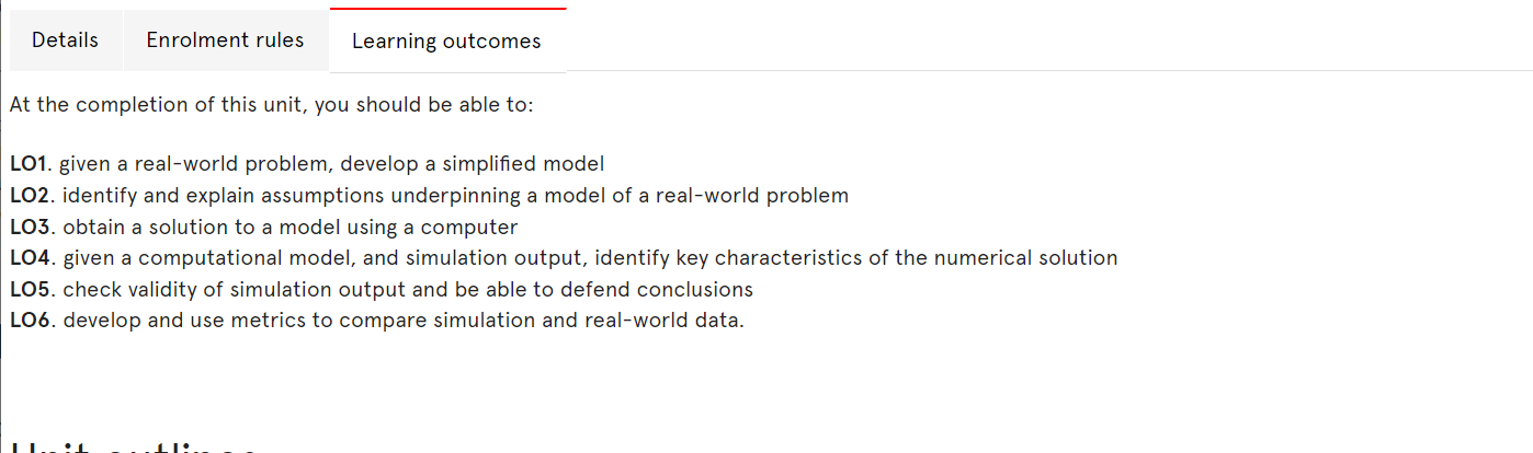
This OLE will provide a general introduction to the research field of quantum computing, covering hardware, software, and potential societal impact. The circuit model of quantum computing and example algorithms will be introduced, then building on this knowledge you will code and execute simple algorithms in a quantum software environment. Emphasis will be given to comparing quantum vs ‘classical’ performance of key algorithms. For hardware, the research challenges in developing quantum computer technology will be introduced, and you will undertake a critical analysis of specific hardware platforms (advantages and challenges). The potential societal impact of quantum computers, and quantum technologies more broadly, will be surveyed. On completion of this OLE, you will have gained an informed appreciation of this new technology and its potential impact, as well as generic skills that allow for the critical assessment and evaluation of potential new technologies.

澳洲代写|OLET2610|Foundations of Quantum Computing量子计算的基础 悉尼大学
AttributeDetail
CodeOLET2610
Academic UnitPhysics Academic Operations
Unit NameFoundations of Quantum Computing
Credit Points2
Pre-requisitesNone mentioned in the provided text
LecturersNot explicitly mentioned in the text

Foundations of Quantum Computing量子计算的基础理论

1.4.3 Reduced Density Matrix
Consider a Hilbert space $\mathcal{H}=\mathcal{H}_A \oplus \mathcal{H}_B$. The reduced density matrix for system $A$ is defined as:
$$
\rho^A \equiv \operatorname{tr}_B\left(\rho^{A B}\right)
$$
$\operatorname{tr}_B$ is known as the partial trace of $\rho^{A B}$ over $B$. The partial trace is defined as :
$$
\operatorname{tr}_B\left(\left|a_1\right\rangle\left\langle a_1|| b_1\right\rangle\left\langle b_2\right|\right) \equiv\left|a_1\right\rangle\left\langle a_1\right| \operatorname{tr}\left(\left|b_1\right\rangle\left\langle b_2\right|\right)
$$
As we expect, if our state is just a tensor product a density matrix $\rho_A$ in $\mathcal{H}_A$ and a density matrix $\rho_B$ in $\mathcal{H}_B$ then
$$
\rho^A=\operatorname{tr}_B\left(\rho_A \rho_B\right)=\rho_A \operatorname{tr}\left(\rho_B\right)=\rho_A
$$
A less trivial example is the bell state.

1.4.6 Example: Infinite Square Well
As an example let us consider a particle sitting in a infinite square well with the state $\psi(x)=\sqrt{\frac{2}{\pi}} \sin (x), x \in[0, \pi]$. The density matrix is:
$$
\rho=\frac{2}{\pi} \sin x^{\prime} \sin x
$$
Now let us break the square well in half into two subspaces, $\mathcal{H}A \otimes \mathcal{H}_B$. Somewhat suprisingly, now we can calculate entropy and entanglement of these subspaces, even though the entire system is pure (and has zero entropy and entanglement). The key difference now is that in each subspace we no longer know if there is a particle or not. Thus, we must express each sub-Hilbert space in the basis $(|0\rangle+|1\rangle) \otimes \psi(x)$ where $|0\rangle$ represents no particle and $|1\rangle$ represents one particle. Equivalently, you can think of this as a way of breaking up the wave function into two functions. $$ \psi=|0,0\rangle \otimes|1, \psi(x)\rangle+|1, \psi(x)\rangle \otimes|0,0\rangle $$ Or, compressing notation and ignoring normalization for now, $$ \psi=|01\rangle+|10\rangle $$ Now we can find the reduced density matrix for $\mathcal{H}_A$. First we rewrite $\rho$ : $$ \begin{aligned} & \rho=(|01\rangle+|10\rangle)(\langle 01|+\langle 10|) \ & \rho=|01\rangle\langle 01|+| 10\rangle\langle 10|+| 10\rangle\langle 01|+| 01\rangle+\langle 10| \end{aligned} $$ The trace of $|10\rangle\langle 01|$ is zero since $\operatorname{tr}(|10\rangle\langle 01|)=\operatorname{tr}(\langle 01 \mid 10\rangle)=0$. We are left with $$ \begin{aligned} & \rho_A=\frac{2}{\pi} \sin x \sin y|1\rangle\left\langle 1\left|+\int{\pi / 2}^\pi \frac{2}{\pi} \sin (x)^2 d x\right| 0\right\rangle\langle 0| \
& \rho_A=\frac{2}{\pi} \sin x \sin y|1\rangle\left\langle 1\left|+\frac{1}{2}\right| 0\right\rangle\langle 0|
\end{aligned}
$$
To calculate the entropy of this subsystem we must know the eigenvalues of $\rho_A$. By inspection, it is clear that $|0\rangle$ is an eigenvector with eigenvalue $\frac{1}{2}$. We know the sum of the eigenvalues must be 1 , so the other eigenvalue is $\frac{1}{2}$. (Alternativly we could try $f(x)|1\rangle$ and work out the corresponding inner product, which is an integral.)
$$
S=-\operatorname{tr}(\rho \ln (\rho))=-\frac{1}{2} \ln \frac{1}{2}-\frac{1}{2} \ln \frac{1}{2}=\ln (2)
$$
This result could have been anticipated because there are two possibilities for measurement – we find the particle on the left or the right. Still, it is suprising that the entropy of a given subsystem can be non-zero while the entire system has zero entropy.

 Quantum Algorithms 量子算法定义

the two possible states of the electron in classical physics. Many of the most counterintuitive aspects of quantum physics arise from the superposition principle which states that if a quantum system can be in one of two states, then it can also be in any linear superposition of those two states. For instance, the state of the electron could well be $\frac{1}{\sqrt{2}}|0\rangle+\frac{1}{\sqrt{2}}|1\rangle$ or $\frac{1}{\sqrt{2}}|0\rangle-\frac{1}{\sqrt{2}}|1\rangle$; or an infinite number of other combinations of the form $\alpha_0|0\rangle+\alpha_1|1\rangle$. The coefficient $\alpha_0$ is called the amplitude of state $|0\rangle$, and similarly with $\alpha_1$. And-if things aren’t already strange enough – the $\alpha$ ‘s can be complex numbers, as long as they are normalized so that $\left|\alpha_0\right|^2+\left|\alpha_1\right|^2=1$. For example, $\frac{1}{\sqrt{5}}|0\rangle+\frac{2 i}{\sqrt{5}}|1\rangle$ (where $i$ is the imaginary unit, $\sqrt{-1}$ ) is a perfectly valid quantum state! Such a superposition, $\alpha_0|0\rangle+\alpha_1|1\rangle$, is the basic unit of encoded information in quantum computers (Figure 10.1). It is called a qubit (pronounced “cubit”).
The whole concept of a superposition suggests that the electron does not make up its mind about whether it is in the ground or excited state, and the amplitude $\alpha_0$ is a measure of its inclination toward the ground state. Continuing along this line of thought, it is tempting to think of $\alpha_0$ as the probability that the electron is in the ground state. But then how are we to make sense of the fact that $\alpha_0$ can be negative, or even worse, imaginary? This is one of the most mysterious aspects of quantum physics, one that seems to extend beyond our intuitions about the physical world.

This linear superposition, however, is the private world of the electron. For us to get a glimpse of the electron’s state we must make a measurement, and when we do so, we get a single bit of information -0 or 1 . If the state of the electron is $\alpha_0|0\rangle+\alpha_1|1\rangle$, then the outcome of the measurement is 0 with probability $\left|\alpha_0\right|^2$ and 1 with probability $\left|\alpha_1\right|^2$ (luckily we normalized so $\left|\alpha_0\right|^2+\left|\alpha_1\right|^2=1$ ). Moreover, the act of measurement causes the system to change its state: if the outcome of the measurement is 0 , then the new state of the system is $|0\rangle$ (the ground state), and if the outcome is 1 , the new state is $|1\rangle$ (the excited state). Thisfeature of quantum physics, that a measurement disturbs the system and forces it to choose (in this case ground or excited state), is another strange phenomenon with no classical analog.

The superposition principle holds not just for 2-level systems like the one we just described, but in general for $k$-level systems. For example, in reality the electron in the hydrogen atom can be in one of many energy levels, starting with the ground state, the first excited state, the second excited state, and so on. So we could consider a $k$-level system consisting of the ground state and the first $k-1$ excited states, and we could denote these by $|0\rangle,|1\rangle,|2\rangle, \ldots,|k-1\rangle$. The superposition principle would then say that the general quantum state of the system is $\alpha_0|0\rangle+\alpha_1|1\rangle+\cdots+\alpha_{k-1}|k-1\rangle$, where $\sum_{j=0}^{k-1}\left|\alpha_j\right|^2=1$. Measuring the state of the system would now reveal a number between 0 and $k-1$, and outcome $j$ would occur with probability $\left|\alpha_j\right|^2$. As before, the measurement would disturb the system, and the new state would actually become $|j\rangle$ or the $j$ th excited state.

How do we encode $n$ bits of information? We could choose $k=2^n$ levels of the hydrogen atom. But a more promising option is to use $n$ qubits.

Let us start by considering the case of two qubits, that is, the state of the electrons of two hydrogen atoms. Since each electron can be in either the ground or excited state, in classical physics the two electrons have a total of four possible states-00, 01, 10, or 11-and are therefore suitable for storing 2 bits of information. But in quantum physics, the superposition principle tells us that the quantum state of the two electrons is a linear combination of the four classical states,
$$
|\boldsymbol{\alpha}\rangle=\alpha_{00}|00\rangle+\alpha_{01}|01\rangle+\alpha_{10}|10\rangle+\alpha_{11}|11\rangle,
$$

澳洲代写|ECOS3022|The Economics of Financial Markets金融市场经济学 悉尼大学

统计代写请认准statistics-lab™. statistics-lab™为您的留学生涯保驾护航。

金融工程代写

金融工程是使用数学技术来解决金融问题。金融工程使用计算机科学、统计学、经济学和应用数学领域的工具和知识来解决当前的金融问题,以及设计新的和创新的金融产品。

非参数统计代写

非参数统计指的是一种统计方法,其中不假设数据来自于由少数参数决定的规定模型;这种模型的例子包括正态分布模型和线性回归模型。

广义线性模型代考

广义线性模型(GLM)归属统计学领域,是一种应用灵活的线性回归模型。该模型允许因变量的偏差分布有除了正态分布之外的其它分布。

术语 广义线性模型(GLM)通常是指给定连续和/或分类预测因素的连续响应变量的常规线性回归模型。它包括多元线性回归,以及方差分析和方差分析(仅含固定效应)。

有限元方法代写

有限元方法(FEM)是一种流行的方法,用于数值解决工程和数学建模中出现的微分方程。典型的问题领域包括结构分析、传热、流体流动、质量运输和电磁势等传统领域。

有限元是一种通用的数值方法,用于解决两个或三个空间变量的偏微分方程(即一些边界值问题)。为了解决一个问题,有限元将一个大系统细分为更小、更简单的部分,称为有限元。这是通过在空间维度上的特定空间离散化来实现的,它是通过构建对象的网格来实现的:用于求解的数值域,它有有限数量的点。边界值问题的有限元方法表述最终导致一个代数方程组。该方法在域上对未知函数进行逼近。[1] 然后将模拟这些有限元的简单方程组合成一个更大的方程系统,以模拟整个问题。然后,有限元通过变化微积分使相关的误差函数最小化来逼近一个解决方案。

tatistics-lab作为专业的留学生服务机构,多年来已为美国、英国、加拿大、澳洲等留学热门地的学生提供专业的学术服务,包括但不限于Essay代写,Assignment代写,Dissertation代写,Report代写,小组作业代写,Proposal代写,Paper代写,Presentation代写,计算机作业代写,论文修改和润色,网课代做,exam代考等等。写作范围涵盖高中,本科,研究生等海外留学全阶段,辐射金融,经济学,会计学,审计学,管理学等全球99%专业科目。写作团队既有专业英语母语作者,也有海外名校硕博留学生,每位写作老师都拥有过硬的语言能力,专业的学科背景和学术写作经验。我们承诺100%原创,100%专业,100%准时,100%满意。

随机分析代写


随机微积分是数学的一个分支,对随机过程进行操作。它允许为随机过程的积分定义一个关于随机过程的一致的积分理论。这个领域是由日本数学家伊藤清在第二次世界大战期间创建并开始的。

时间序列分析代写

随机过程,是依赖于参数的一组随机变量的全体,参数通常是时间。 随机变量是随机现象的数量表现,其时间序列是一组按照时间发生先后顺序进行排列的数据点序列。通常一组时间序列的时间间隔为一恒定值(如1秒,5分钟,12小时,7天,1年),因此时间序列可以作为离散时间数据进行分析处理。研究时间序列数据的意义在于现实中,往往需要研究某个事物其随时间发展变化的规律。这就需要通过研究该事物过去发展的历史记录,以得到其自身发展的规律。

回归分析代写

多元回归分析渐进(Multiple Regression Analysis Asymptotics)属于计量经济学领域,主要是一种数学上的统计分析方法,可以分析复杂情况下各影响因素的数学关系,在自然科学、社会和经济学等多个领域内应用广泛。

MATLAB代写

MATLAB 是一种用于技术计算的高性能语言。它将计算、可视化和编程集成在一个易于使用的环境中,其中问题和解决方案以熟悉的数学符号表示。典型用途包括:数学和计算算法开发建模、仿真和原型制作数据分析、探索和可视化科学和工程图形应用程序开发,包括图形用户界面构建MATLAB 是一个交互式系统,其基本数据元素是一个不需要维度的数组。这使您可以解决许多技术计算问题,尤其是那些具有矩阵和向量公式的问题,而只需用 C 或 Fortran 等标量非交互式语言编写程序所需的时间的一小部分。MATLAB 名称代表矩阵实验室。MATLAB 最初的编写目的是提供对由 LINPACK 和 EISPACK 项目开发的矩阵软件的轻松访问,这两个项目共同代表了矩阵计算软件的最新技术。MATLAB 经过多年的发展,得到了许多用户的投入。在大学环境中,它是数学、工程和科学入门和高级课程的标准教学工具。在工业领域,MATLAB 是高效研究、开发和分析的首选工具。MATLAB 具有一系列称为工具箱的特定于应用程序的解决方案。对于大多数 MATLAB 用户来说非常重要,工具箱允许您学习应用专业技术。工具箱是 MATLAB 函数(M 文件)的综合集合,可扩展 MATLAB 环境以解决特定类别的问题。可用工具箱的领域包括信号处理、控制系统、神经网络、模糊逻辑、小波、仿真等。

R语言代写问卷设计与分析代写
PYTHON代写回归分析与线性模型代写
MATLAB代写方差分析与试验设计代写
STATA代写机器学习/统计学习代写
SPSS代写计量经济学代写
EVIEWS代写时间序列分析代写
EXCEL代写深度学习代写
SQL代写各种数据建模与可视化代写

澳洲代写|COMP5328|Advanced Machine Learning高级机器学习 悉尼大学

statistics-labTM为您悉尼大学(英语:The University of Sydney)Advanced Machine Learning高级机器学习澳洲代写代考辅导服务!

课程介绍:

Machine learning models explain and generalise data. This course introduces some fundamental machine learning concepts, learning problems and algorithms to provide understanding and simple answers to many questions arising from data explanation and generalisation. For example, why do different machine learning models work? How to further improve them? How to adapt them to different purposes?

澳洲代写|COMP5328|Advanced Machine Learning高级机器学习 悉尼大学
AttributeDetail
Year/SessionSemester 2, 2020
CodeCOMP5328
Academic UnitComputer Science
Unit NameAdvanced Machine Learning
Credit Points6
Pre-requisitesNone
LecturersNot explicitly mentioned in the text

Advanced Machine Learning高级机器学习理论

Definition: $\operatorname{AR}(p)$ model is a linear generative model based on the $p$ th order Markov assumption:
$$
\forall t, Y_t=\sum_{i=1}^p a_i Y_{t-i}+\epsilon_t
$$
where

$\epsilon_t \mathrm{~s}$ are zero mean uncorrelated random variables with variance $\sigma$.

$a_1, \ldots, a_p$ are autoregressive coefficients.

$Y_t$ is observed stochastic process.

Definition: the generalized autoregressive conditional heteroscedasticity $\operatorname{GARCH}(p, q)$ model is an $\operatorname{ARMA}(p, q)$ model for the variance $\sigma_t$ of the noise term $\epsilon_t$ :

$$\forall t, \sigma_{t+1}^2=\omega+\sum_{i=0}^{p-1} \alpha_i \sigma_{t-i}^2+\sum_{j=0}^{q-1} \beta_j \epsilon_{t-j}^2$$

where

$\epsilon_t \mathrm{~S}$ are zero mean Gaussian random variables with variance $\sigma_t$ conditioned on $\left{Y_{t-1}, Y_{t-2}, \ldots\right}$.

$\omega>0$ is the mean parameter.

Continuous state space version of Hidden Markov Models:

$$\begin{aligned}\mathbf{X}_{t+1} & =\mathbf{B X}_t+\mathbf{U}_t, \Y_t & =\mathbf{A} \mathbf{X}_t+\epsilon_t\end{aligned}$$where$\mathbf{X}_t$ is an $n$-dimensional state vector.$Y_t$ is an observed stochastic process.$\mathbf{A}$ and $\mathbf{B}$ are model parameters.$\mathbf{U}_t$ and $\epsilon_t$ are noise terms.

Different methods for estimating model parameters:

  • Maximum likelihood estimation:
  • Requires further parametric assumptions on the noise distribution (e.g. Gaussian).
  • Method of moments (Yule-Walker estimator).
  • Conditional and unconditional least square estimation.
  • Restricted to certain models.

 Complexity and Generalisation复杂性和概括性 定义

Given a space $Z$ and a fixed distribution $\left.D\right|Z$, let $S=\left{z_1, \ldots, z_m\right}$ be a set of examples drawn i.i.d. from $\left.D\right|_Z$. Furthermore, let $\mathcal{F}$ be a class of functions $f: Z \rightarrow \mathbb{R}$. Definition. The empirical Rademacher complexity of $\mathcal{F}$ is defined to be $$ \hat{R}_m(\mathcal{F})=\mathrm{E}\sigma\left[\sup {f \in \mathcal{F}}\left(\frac{1}{m} \sum{i=1}^m \sigma_i f\left(z_i\right)\right)\right]
$$
where $\sigma_1, \ldots, \sigma_m$ are independent random variables uniformly chosen from ${-1,1}$. We will refer to such random variables as Rademacher variables.
Definition. The Rademacher complexity of $\mathcal{F}$ is defined as
$$
R_m(\mathcal{F})=\mathrm{E}_D\left[\hat{R}_m(\mathcal{F})\right]
$$

Intuitively, the supremum measures, for a given set $S$ and Rademacher vector $\sigma$, the maximum correlation between $f\left(z_i\right)$ and $\sigma_i$ over all $f \in \mathcal{F}$. Taking the expectation over $\sigma$, we can then say that the empirical Rademacher complexity of $\mathcal{F}$ measures the ability of functions from $\mathcal{F}$ (when applied to a fixed set $S$ ) to fit random noise. The Rademacher complexity of $\mathcal{F}$ then measures the expected noise-fitting-ability of $\mathcal{F}$ over all data sets $S \in Z^m$ that could be drawn according to the distribution $\left.D\right|_Z$.

We note that Rademacher complexity can be defined even more generally on sets $A \subseteq \mathbb{R}^m$ by making the supremum over $a \in A$ (instead of $f \in \mathcal{F}$ ) and replacing each $f\left(z_i\right)$ with $a_i$. Taking $A=\mathcal{F}(S)={f(z) \mid f \in \mathcal{F}, z \in S}$ recovers the definition above. It will sometimes be convenient to use the more general definition.

澳洲代写|ECOS3022|The Economics of Financial Markets金融市场经济学 悉尼大学

统计代写请认准statistics-lab™. statistics-lab™为您的留学生涯保驾护航。

金融工程代写

金融工程是使用数学技术来解决金融问题。金融工程使用计算机科学、统计学、经济学和应用数学领域的工具和知识来解决当前的金融问题,以及设计新的和创新的金融产品。

非参数统计代写

非参数统计指的是一种统计方法,其中不假设数据来自于由少数参数决定的规定模型;这种模型的例子包括正态分布模型和线性回归模型。

广义线性模型代考

广义线性模型(GLM)归属统计学领域,是一种应用灵活的线性回归模型。该模型允许因变量的偏差分布有除了正态分布之外的其它分布。

术语 广义线性模型(GLM)通常是指给定连续和/或分类预测因素的连续响应变量的常规线性回归模型。它包括多元线性回归,以及方差分析和方差分析(仅含固定效应)。

有限元方法代写

有限元方法(FEM)是一种流行的方法,用于数值解决工程和数学建模中出现的微分方程。典型的问题领域包括结构分析、传热、流体流动、质量运输和电磁势等传统领域。

有限元是一种通用的数值方法,用于解决两个或三个空间变量的偏微分方程(即一些边界值问题)。为了解决一个问题,有限元将一个大系统细分为更小、更简单的部分,称为有限元。这是通过在空间维度上的特定空间离散化来实现的,它是通过构建对象的网格来实现的:用于求解的数值域,它有有限数量的点。边界值问题的有限元方法表述最终导致一个代数方程组。该方法在域上对未知函数进行逼近。[1] 然后将模拟这些有限元的简单方程组合成一个更大的方程系统,以模拟整个问题。然后,有限元通过变化微积分使相关的误差函数最小化来逼近一个解决方案。

tatistics-lab作为专业的留学生服务机构,多年来已为美国、英国、加拿大、澳洲等留学热门地的学生提供专业的学术服务,包括但不限于Essay代写,Assignment代写,Dissertation代写,Report代写,小组作业代写,Proposal代写,Paper代写,Presentation代写,计算机作业代写,论文修改和润色,网课代做,exam代考等等。写作范围涵盖高中,本科,研究生等海外留学全阶段,辐射金融,经济学,会计学,审计学,管理学等全球99%专业科目。写作团队既有专业英语母语作者,也有海外名校硕博留学生,每位写作老师都拥有过硬的语言能力,专业的学科背景和学术写作经验。我们承诺100%原创,100%专业,100%准时,100%满意。

随机分析代写


随机微积分是数学的一个分支,对随机过程进行操作。它允许为随机过程的积分定义一个关于随机过程的一致的积分理论。这个领域是由日本数学家伊藤清在第二次世界大战期间创建并开始的。

时间序列分析代写

随机过程,是依赖于参数的一组随机变量的全体,参数通常是时间。 随机变量是随机现象的数量表现,其时间序列是一组按照时间发生先后顺序进行排列的数据点序列。通常一组时间序列的时间间隔为一恒定值(如1秒,5分钟,12小时,7天,1年),因此时间序列可以作为离散时间数据进行分析处理。研究时间序列数据的意义在于现实中,往往需要研究某个事物其随时间发展变化的规律。这就需要通过研究该事物过去发展的历史记录,以得到其自身发展的规律。

回归分析代写

多元回归分析渐进(Multiple Regression Analysis Asymptotics)属于计量经济学领域,主要是一种数学上的统计分析方法,可以分析复杂情况下各影响因素的数学关系,在自然科学、社会和经济学等多个领域内应用广泛。

MATLAB代写

MATLAB 是一种用于技术计算的高性能语言。它将计算、可视化和编程集成在一个易于使用的环境中,其中问题和解决方案以熟悉的数学符号表示。典型用途包括:数学和计算算法开发建模、仿真和原型制作数据分析、探索和可视化科学和工程图形应用程序开发,包括图形用户界面构建MATLAB 是一个交互式系统,其基本数据元素是一个不需要维度的数组。这使您可以解决许多技术计算问题,尤其是那些具有矩阵和向量公式的问题,而只需用 C 或 Fortran 等标量非交互式语言编写程序所需的时间的一小部分。MATLAB 名称代表矩阵实验室。MATLAB 最初的编写目的是提供对由 LINPACK 和 EISPACK 项目开发的矩阵软件的轻松访问,这两个项目共同代表了矩阵计算软件的最新技术。MATLAB 经过多年的发展,得到了许多用户的投入。在大学环境中,它是数学、工程和科学入门和高级课程的标准教学工具。在工业领域,MATLAB 是高效研究、开发和分析的首选工具。MATLAB 具有一系列称为工具箱的特定于应用程序的解决方案。对于大多数 MATLAB 用户来说非常重要,工具箱允许您学习应用专业技术。工具箱是 MATLAB 函数(M 文件)的综合集合,可扩展 MATLAB 环境以解决特定类别的问题。可用工具箱的领域包括信号处理、控制系统、神经网络、模糊逻辑、小波、仿真等。

R语言代写问卷设计与分析代写
PYTHON代写回归分析与线性模型代写
MATLAB代写方差分析与试验设计代写
STATA代写机器学习/统计学习代写
SPSS代写计量经济学代写
EVIEWS代写时间序列分析代写
EXCEL代写深度学习代写
SQL代写各种数据建模与可视化代写

澳洲代写|ECOS3022|The Economics of Financial Markets金融市场经济学 悉尼大学

statistics-labTM为您悉尼大学(英语:The University of Sydney)The Economics of Financial Markets金融市场经济学 澳洲代写代考辅导服务!

课程介绍:

Financial assets play a vital role coordinating the actions of savers and investors; consequently, they play a crucial role in creating wealth and facilitating economic activity. The aim of this unit is to explore the economic principles underlying: the pricing and development of financial assets; the trade-off between risk and return and the how investors construct portfolios in response to this trade-off. The focus is on the economics of financial markets: the factors of demand and supply; risk and uncertainty; incomplete contracts and renegotiation; and asymmetric information and its implications. We will emphasize the key aspects of markets for financial assets and the main differences to markets for consumption goods. The unit also examines the development of financial institutions and current issues in financial markets.

ECON1001|Introductory Microeconomics微观经济学入门 悉尼大学
AttributeDetail
Course CodeECOS3022
Academic UnitEconomics
Unit NameThe Economics of Financial Markets
Credit Points6

The Economics of Financial Markets金融市场经济学 案例

问题 1.

Suppose each agent’s utility function is continuous and strongly monotone. Then an allocation $x^*$ is Pareto optimal if and only if it is a solution to (A) for some choice of $\left{\bar{U}i\right}{i \neq j}$.

Proof. We first prove sufficiency: if $x$ Pareto optimal, then it solves (eq:planner) for $\bar{U}_i=U_i\left(x_i\right)$. Take any feasible argument $y=\left(y_1, \ldots, y_m\right)$ for (A). Considering the constraints, $U_i\left(y_i\right) \geq U_i\left(x_i\right)$ and $y$ is an allocation. So $U_1\left(y_j\right) \leq U_1\left(x_1\right)$, as otherwise $y$ would Pareto dominate $x$. Since this is true of any feasible alternative, $x$ is a solution to (A).

We not prove the necessity direction contrapositively. Suppose $x$ is Pareto dominated by $y$. There are two possible cases. Case 1: $U_1\left(y_1\right)>U_1\left(x_1\right)$. Whenever $x$ is feasible for (eq:planner), $y$ is feasible as well. But since $y$ strictly improves the objective, $x$ cannot be a solution. Case 2: $U_1\left(y_1\right)=U_1\left(x_1\right)$. Then there must exist some agent $k \neq 1$ such that $U_k\left(y_k\right)>U_k\left(x_k\right)$. Without loss of generality, let $k=2$. Since $U_2$ is continuous, the strict inequality is maintained in a neighborhood of $y_2$. So for sufficiently small $\delta>0, U_2\left((1-\delta) y_2\right)>U_2\left(x_2\right)$. Moreover, since $U_1$ is strongly monotone, $U_1\left(y_1+\delta y_2\right)>U_1\left(y_1\right)=U_1\left(x_1\right)$. Then $\left(y_1+\delta y_2,(1-\delta) y_2, y_3, \ldots, y_m\right)$ is an allocation that Pareto dominates $x$ and $U_1\left(y_1+\delta y_2\right)>U_1\left(x_1\right)$. Now apply Case 1 .

The characterization yields a geometric interpretation of Pareto optimality. Specifically, consider the first-order conditions for (A). The following is necessary for any allocation $x^$ to be an interior Pareto optimal allocation: $$ D U_i\left(x_i^\right)=\lambda_j D U_j\left(x_j^\right) $$ for some set of Lagrange multipliers $\lambda_j$. That is, the tangent of agent $i$ ‘s indifference curve $x_i^$ is identical to agent $j$ ‘s. In particular, the ratio of the partial derivatives of any two goods $\ell, \ell^{\prime}$ are identical:
$$
\left.\frac{\partial U_i / \partial x_{i \ell}}{\partial U_i / \partial x_{i \ell^{\prime}}}\right|{x_i=x_i^}=\left.\frac{\partial U_i / \partial x{j \ell}}{\partial U_i / \partial x_{j \ell^{\prime}}}\right|_{x_j=x_j^}
$$
In other words, the marginal rates of substitution of $\ell$ to $\ell^{\prime}$ are identical across agents. Considering the standard calculus characterization of marginal rates of substitution in terms of price, this may or may not be surprising for anyone who recalls her intermediate microeconomics course.

问题 2. If each $U_i$ is strongly monotone, then every competitive equilibrium allocation in an exchange economy is Pareto optimal

Proof. Let $x^=\left(x_1^, \ldots, x_m^\right)$ be an equilibrium allocation with corresponding equilibrium price $p^$. Consider any allocation $y=\left(y_1, \ldots, y_m\right)$ that Pareto dominates $x^$. Without loss of generality, suppose $U_1\left(y_1\right)>U_1\left(x_1^\right)$ and $U_i\left(y_i\right) \geq U_i\left(x_i^\right)$ for all $i>1$. Then $$ p^ \cdot y_1>p^* \cdot x_1^, $$ because $x_1^$ is optimal for the agent 1’s problem, so any improving $y_1$ is infeasible. Since $U_i\left(y_i\right) \geq$ $U_i\left(x_i^\right)$ and $x_i$ is optimal for agent $i$ ‘s problem, we know $y_i$ is also optimal for agent $i$ ‘s problem. The budget constraint must therefore be binding at $y_i$ by strong monotonicity. Hence $$ p^ \cdot y_i=p^* \cdot \omega_i .
$$
By adding these relations,
$$
p^* \cdot \sum_i y_i>p^* \cdot \sum_i x_i=p \cdot \omega .
$$
Thus $\sum_i y_i>\omega$, that is, $y$ is not feasible. Since any Pareto dominating allocation is infeasible, $x^*$ is Pareto optimal.

In fact, strong monotonicity of utility can be relaxed. As long as individual demand satisfies Walras’s Law, that is, $p \cdot x_i=p \cdot \omega$ whenever $x_i$ is a optimal for the agent’s problem at price $p$, the First Welfare Theorem holds.

The Economics of Financial Markets金融市场经济学 定义

Recall the following vector notation: For $x, y \in \mathbb{R}^L$, we write:

  • $x \geq y$ if $x_{\ell} \geq y_{\ell}$ for all $\ell=1, \ldots, L$;
  • $x>y$ if $x \geq y$ and $x \neq y$;
  • $x \gg y$ if $x_{\ell}>y_{\ell}$ for all $\ell=1, \ldots, L$.
    Definition 1.1. An exchange economy consists of:
  • $L$ commodities $(\ell=1, \ldots, L)$ which form a commodity space $\mathbb{R}_{+}^L$
  • $m$ agents $(i=1, \ldots, m)$ where each agent has
  • a preference relation $\succsim_i$ over $\mathbb{R}{+}^L$ (or utility function $U_i: \mathbb{R}{+}^L \rightarrow \mathbb{R}$
  • a vector of initial endowments $\omega_i \in \mathbb{R}_{+}^L$
    We will often assume that the preference relation admits a utility representation that is strongly monotone: $\left(x>x^{\prime}\right.$ implies $\left.x \succ_i x^{\prime}\right)$, continuous, and quasi-concave.

Definition 1.2. Let $\omega=\sum_{i=1}^n \omega_i$ denote the social endowment. An allocation in an exchange economy is an assignment of goods to agents $x=\left(x_1, \ldots, x_m\right) \in\left(\mathbb{R}{+}^L\right)^n$. An allocation is feasible if $$ \sum{i=1}^m x_i=\omega .
$$
Definition 1.3. We write that allocation $y$ Pareto dominates allocation $x$ if $y_i \succsim_i x_i$ for all $i$ and $y_j \succ_i x_j$ for some $j$ (or equivalently, $\left(U_1\left(y_1\right), \ldots U_n\left(y_n\right)\right)>\left(U_1\left(x_1\right), \ldots, U_n\left(x_n\right)\right)$ A feasible allocation $x^$ is Pareto optimal if there is no other feasible allocation $x$ that Pareto dominates $x^$.

When agents’ preferences are continuous and strongly monotone, the set of Pareto optimal feasible allocations can be parameterized through a family of maximization problems. Specifically, consider the following constrained program, parameterized by a choice of minimal utility levels $\bar{U}i$ for all $i>1$ : $$ \begin{array}{ll} \underset{\left(x_1, \ldots, x_m\right)}{\operatorname{maximize}} & U_1\left(x_1\right) \ \text { subject to } & U_i\left(x_i\right) \geq \bar{U}_i, \forall i>1 \ & \sum{i=1}^m x_i=\omega \
& x_i \geq 0, \forall i .
\end{array}
$$

澳洲代写|ECOS3022|The Economics of Financial Markets金融市场经济学 悉尼大学

统计代写请认准statistics-lab™. statistics-lab™为您的留学生涯保驾护航。

金融工程代写

金融工程是使用数学技术来解决金融问题。金融工程使用计算机科学、统计学、经济学和应用数学领域的工具和知识来解决当前的金融问题,以及设计新的和创新的金融产品。

非参数统计代写

非参数统计指的是一种统计方法,其中不假设数据来自于由少数参数决定的规定模型;这种模型的例子包括正态分布模型和线性回归模型。

广义线性模型代考

广义线性模型(GLM)归属统计学领域,是一种应用灵活的线性回归模型。该模型允许因变量的偏差分布有除了正态分布之外的其它分布。

术语 广义线性模型(GLM)通常是指给定连续和/或分类预测因素的连续响应变量的常规线性回归模型。它包括多元线性回归,以及方差分析和方差分析(仅含固定效应)。

有限元方法代写

有限元方法(FEM)是一种流行的方法,用于数值解决工程和数学建模中出现的微分方程。典型的问题领域包括结构分析、传热、流体流动、质量运输和电磁势等传统领域。

有限元是一种通用的数值方法,用于解决两个或三个空间变量的偏微分方程(即一些边界值问题)。为了解决一个问题,有限元将一个大系统细分为更小、更简单的部分,称为有限元。这是通过在空间维度上的特定空间离散化来实现的,它是通过构建对象的网格来实现的:用于求解的数值域,它有有限数量的点。边界值问题的有限元方法表述最终导致一个代数方程组。该方法在域上对未知函数进行逼近。[1] 然后将模拟这些有限元的简单方程组合成一个更大的方程系统,以模拟整个问题。然后,有限元通过变化微积分使相关的误差函数最小化来逼近一个解决方案。

tatistics-lab作为专业的留学生服务机构,多年来已为美国、英国、加拿大、澳洲等留学热门地的学生提供专业的学术服务,包括但不限于Essay代写,Assignment代写,Dissertation代写,Report代写,小组作业代写,Proposal代写,Paper代写,Presentation代写,计算机作业代写,论文修改和润色,网课代做,exam代考等等。写作范围涵盖高中,本科,研究生等海外留学全阶段,辐射金融,经济学,会计学,审计学,管理学等全球99%专业科目。写作团队既有专业英语母语作者,也有海外名校硕博留学生,每位写作老师都拥有过硬的语言能力,专业的学科背景和学术写作经验。我们承诺100%原创,100%专业,100%准时,100%满意。

随机分析代写


随机微积分是数学的一个分支,对随机过程进行操作。它允许为随机过程的积分定义一个关于随机过程的一致的积分理论。这个领域是由日本数学家伊藤清在第二次世界大战期间创建并开始的。

时间序列分析代写

随机过程,是依赖于参数的一组随机变量的全体,参数通常是时间。 随机变量是随机现象的数量表现,其时间序列是一组按照时间发生先后顺序进行排列的数据点序列。通常一组时间序列的时间间隔为一恒定值(如1秒,5分钟,12小时,7天,1年),因此时间序列可以作为离散时间数据进行分析处理。研究时间序列数据的意义在于现实中,往往需要研究某个事物其随时间发展变化的规律。这就需要通过研究该事物过去发展的历史记录,以得到其自身发展的规律。

回归分析代写

多元回归分析渐进(Multiple Regression Analysis Asymptotics)属于计量经济学领域,主要是一种数学上的统计分析方法,可以分析复杂情况下各影响因素的数学关系,在自然科学、社会和经济学等多个领域内应用广泛。

MATLAB代写

MATLAB 是一种用于技术计算的高性能语言。它将计算、可视化和编程集成在一个易于使用的环境中,其中问题和解决方案以熟悉的数学符号表示。典型用途包括:数学和计算算法开发建模、仿真和原型制作数据分析、探索和可视化科学和工程图形应用程序开发,包括图形用户界面构建MATLAB 是一个交互式系统,其基本数据元素是一个不需要维度的数组。这使您可以解决许多技术计算问题,尤其是那些具有矩阵和向量公式的问题,而只需用 C 或 Fortran 等标量非交互式语言编写程序所需的时间的一小部分。MATLAB 名称代表矩阵实验室。MATLAB 最初的编写目的是提供对由 LINPACK 和 EISPACK 项目开发的矩阵软件的轻松访问,这两个项目共同代表了矩阵计算软件的最新技术。MATLAB 经过多年的发展,得到了许多用户的投入。在大学环境中,它是数学、工程和科学入门和高级课程的标准教学工具。在工业领域,MATLAB 是高效研究、开发和分析的首选工具。MATLAB 具有一系列称为工具箱的特定于应用程序的解决方案。对于大多数 MATLAB 用户来说非常重要,工具箱允许您学习应用专业技术。工具箱是 MATLAB 函数(M 文件)的综合集合,可扩展 MATLAB 环境以解决特定类别的问题。可用工具箱的领域包括信号处理、控制系统、神经网络、模糊逻辑、小波、仿真等。

R语言代写问卷设计与分析代写
PYTHON代写回归分析与线性模型代写
MATLAB代写方差分析与试验设计代写
STATA代写机器学习/统计学习代写
SPSS代写计量经济学代写
EVIEWS代写时间序列分析代写
EXCEL代写深度学习代写
SQL代写各种数据建模与可视化代写

FMHU5002|Introductory Biostatistics生物统计学导论 悉尼大学

statistics-labTM为您悉尼大学(英语:The University of Sydney)Introductory Biostatistics生物统计学导论 澳洲代写代考辅导服务!

课程介绍:

This unit introduces students to statistical methods relevant in medicine and health. Students will learn how to build datasets and basic data management procedures, summarise and visualise data, choose the correct statistical analysis, conduct this analysis using statistical software, interpret its results, and report statistical findings in a format suitable for inclusion in scientific publications. Students will also learn to consider the difference between statistical significance and practical importance, and how to determine the appropriate sample size when planning a research study. Specific analysis methods covered in this unit include: descriptive methods; hypothesis tests for one sample, paired samples and two independent groups for continuous and categorical data; correlation and linear regression; power and sample size estimation for simple studies. All these topics are introduced with an emphasis on practical application and interpretation and are supported using statistical software. The general principles developed in this unit can be easily extended to more advanced methods; students who wish to continue with their statistical learning after this unit are encouraged to take PUBH5217 Biostatistics: Statistical Modelling.

ECON1001|Introductory Microeconomics微观经济学入门 悉尼大学

Introductory Biostatistics生物统计学导论 案例

问题 1.

What is the probability that 2 cases of COVID- 19 will be reported in a given day?

Solution:
$$
\begin{aligned}
& \mathrm{P}(\mathrm{X}=\mathrm{x})=\frac{e^{-\lambda} \lambda{ }^x}{X !} \
& \mathrm{P}(\mathrm{X}=\mathrm{x})=\frac{\left(e^{-6.5}\right) 6.5^2}{2 !}=0.0635203059 / 2=0.031760153
\end{aligned}
$$

问题 2. Find a $95 \%$ C.I for the difference of mean height of adult men and women.

$\overline{X_1}-\overline{X_2} \pm Z_{a 2}\left(\sqrt{\frac{\sigma 1^2}{n 1}+\frac{\sigma 2^2}{n 2}}\right)=170-164 \pm 1.96\left(\sqrt{\frac{8^2}{128}+\frac{6^2}{100}}\right)$

$$
\begin{aligned}
& 170-164 \pm 1.96\left(\sqrt{\frac{8^2}{128}+\frac{6^2}{100}}\right)=6 \pm 1.96\left(\sqrt{\frac{64}{128}+\frac{36}{100}}\right)=6 \pm 1.96(\sqrt{0.5+0.36}) \
& 170-164 \pm 1.96\left(\sqrt{\frac{8^2}{128}+\frac{6^2}{100}}\right)=6 \pm 1.96(\sqrt{0.86})=6 \pm 1.96(0.927)=6 \pm 1.81692 \
& 6 \pm 1.81692=(6-1.81692,6+1.81692)=(4.18308,7.81692)
\end{aligned}
$$
Therefore, the $95 \%$ C.I for the difference of mean height of adult men and women is $(4.18308,7.81692)$.

FMHU5002|Introductory Biostatistics生物统计学导论 悉尼大学

统计代写请认准statistics-lab™. statistics-lab™为您的留学生涯保驾护航。

金融工程代写

金融工程是使用数学技术来解决金融问题。金融工程使用计算机科学、统计学、经济学和应用数学领域的工具和知识来解决当前的金融问题,以及设计新的和创新的金融产品。

非参数统计代写

非参数统计指的是一种统计方法,其中不假设数据来自于由少数参数决定的规定模型;这种模型的例子包括正态分布模型和线性回归模型。

广义线性模型代考

广义线性模型(GLM)归属统计学领域,是一种应用灵活的线性回归模型。该模型允许因变量的偏差分布有除了正态分布之外的其它分布。

术语 广义线性模型(GLM)通常是指给定连续和/或分类预测因素的连续响应变量的常规线性回归模型。它包括多元线性回归,以及方差分析和方差分析(仅含固定效应)。

有限元方法代写

有限元方法(FEM)是一种流行的方法,用于数值解决工程和数学建模中出现的微分方程。典型的问题领域包括结构分析、传热、流体流动、质量运输和电磁势等传统领域。

有限元是一种通用的数值方法,用于解决两个或三个空间变量的偏微分方程(即一些边界值问题)。为了解决一个问题,有限元将一个大系统细分为更小、更简单的部分,称为有限元。这是通过在空间维度上的特定空间离散化来实现的,它是通过构建对象的网格来实现的:用于求解的数值域,它有有限数量的点。边界值问题的有限元方法表述最终导致一个代数方程组。该方法在域上对未知函数进行逼近。[1] 然后将模拟这些有限元的简单方程组合成一个更大的方程系统,以模拟整个问题。然后,有限元通过变化微积分使相关的误差函数最小化来逼近一个解决方案。

tatistics-lab作为专业的留学生服务机构,多年来已为美国、英国、加拿大、澳洲等留学热门地的学生提供专业的学术服务,包括但不限于Essay代写,Assignment代写,Dissertation代写,Report代写,小组作业代写,Proposal代写,Paper代写,Presentation代写,计算机作业代写,论文修改和润色,网课代做,exam代考等等。写作范围涵盖高中,本科,研究生等海外留学全阶段,辐射金融,经济学,会计学,审计学,管理学等全球99%专业科目。写作团队既有专业英语母语作者,也有海外名校硕博留学生,每位写作老师都拥有过硬的语言能力,专业的学科背景和学术写作经验。我们承诺100%原创,100%专业,100%准时,100%满意。

随机分析代写


随机微积分是数学的一个分支,对随机过程进行操作。它允许为随机过程的积分定义一个关于随机过程的一致的积分理论。这个领域是由日本数学家伊藤清在第二次世界大战期间创建并开始的。

时间序列分析代写

随机过程,是依赖于参数的一组随机变量的全体,参数通常是时间。 随机变量是随机现象的数量表现,其时间序列是一组按照时间发生先后顺序进行排列的数据点序列。通常一组时间序列的时间间隔为一恒定值(如1秒,5分钟,12小时,7天,1年),因此时间序列可以作为离散时间数据进行分析处理。研究时间序列数据的意义在于现实中,往往需要研究某个事物其随时间发展变化的规律。这就需要通过研究该事物过去发展的历史记录,以得到其自身发展的规律。

回归分析代写

多元回归分析渐进(Multiple Regression Analysis Asymptotics)属于计量经济学领域,主要是一种数学上的统计分析方法,可以分析复杂情况下各影响因素的数学关系,在自然科学、社会和经济学等多个领域内应用广泛。

MATLAB代写

MATLAB 是一种用于技术计算的高性能语言。它将计算、可视化和编程集成在一个易于使用的环境中,其中问题和解决方案以熟悉的数学符号表示。典型用途包括:数学和计算算法开发建模、仿真和原型制作数据分析、探索和可视化科学和工程图形应用程序开发,包括图形用户界面构建MATLAB 是一个交互式系统,其基本数据元素是一个不需要维度的数组。这使您可以解决许多技术计算问题,尤其是那些具有矩阵和向量公式的问题,而只需用 C 或 Fortran 等标量非交互式语言编写程序所需的时间的一小部分。MATLAB 名称代表矩阵实验室。MATLAB 最初的编写目的是提供对由 LINPACK 和 EISPACK 项目开发的矩阵软件的轻松访问,这两个项目共同代表了矩阵计算软件的最新技术。MATLAB 经过多年的发展,得到了许多用户的投入。在大学环境中,它是数学、工程和科学入门和高级课程的标准教学工具。在工业领域,MATLAB 是高效研究、开发和分析的首选工具。MATLAB 具有一系列称为工具箱的特定于应用程序的解决方案。对于大多数 MATLAB 用户来说非常重要,工具箱允许您学习应用专业技术。工具箱是 MATLAB 函数(M 文件)的综合集合,可扩展 MATLAB 环境以解决特定类别的问题。可用工具箱的领域包括信号处理、控制系统、神经网络、模糊逻辑、小波、仿真等。

R语言代写问卷设计与分析代写
PYTHON代写回归分析与线性模型代写
MATLAB代写方差分析与试验设计代写
STATA代写机器学习/统计学习代写
SPSS代写计量经济学代写
EVIEWS代写时间序列分析代写
EXCEL代写深度学习代写
SQL代写各种数据建模与可视化代写

ECON1001|Introductory Microeconomics微观经济学入门 悉尼大学

statistics-labTM为您悉尼大学(英语:The University of Sydney)Introductory Microeconomics微观经济学入门澳洲代写代考辅导服务!

课程介绍:

Introductory Microeconomics addresses the economic decisions of individual firms and households and how these interact in markets. Economic issues are pervasive in contemporary Australian society. Introductory Microeconomics introduces students to the language and analytical framework adopted in Economics for the examination of social phenomena and public policy issues. Whatever one’s career intentions, coming to grips with economic ideas is essential for understanding society, business and government. Students are given a comprehensive introduction to these ideas and are prepared for the advanced study of microeconomics in subsequent years. Prior knowledge of mathematics is assumed.

ECON1001|Introductory Microeconomics微观经济学入门 悉尼大学

Introductory Microeconomics微观经济学入门案例

问题 1.

The NE is $a_1=\frac{32}{15}, a_2=\frac{38}{15}$ (found by solving the two best response functions simultaneously).

(h) Find the Nash equilibrium of the simultaneous move game where player 1 chooses $a_1 \in \Re$, player 2 chooses $a_2 \in \Re$, and the payoffs are
$$
u_1\left(a_1, a_2\right)=-\left(a_1-1\right)^2-\left(a_1-\frac{a_2+2}{2}\right)^2
$$
and
$$
u_2\left(a_1, a_2\right)=-\left(a_2-3\right)^2-\left(a_2-\frac{a_1+2}{2}\right)^2 .
$$
(i) Suppose that in class I presented the following slight variant on Spence’s job market signalling model. Nature first chooses the ability $\theta \in{2,3}$ of player 1 (with both choices being equally likely). Player 1 observes $\theta$ and chooses $e \in{0,1}$. Player 2 then observes $e$ and chooses $w \in \Re$. The players’ utility functions are $u_1(e, w ; \theta)=w-c e / \theta^2$ and $u_2(e, w ; \theta)=-(w-\theta)^2$. For $c=4.25$ this model has both a pooling equilibrium:
$$
\begin{array}{ll}
s_1^(\theta=2)=0 & s_2^(e=0)=2.5 \
s_1^(\theta=3)=0 & s_2^(e=1)=2
\end{array}
$$
$$
\mu_2(\theta=2 \mid e=0)=0.5
$$
$$
\mu_2(\theta=2 \mid e=1)=1
$$
and a separating equilibrium:
$$
\begin{array}{lll}
s_1^(\theta=2)=0 & s_2^(e=0)=2 & \mu_2(\theta=2 \mid e=0)=1 \
s_1^(\theta=3)=1 & s_2^(e=1)=3 & \mu_2(\theta=2 \mid e=1)=0
\end{array}
$$
Suppose that after class two students come up to you in the hallway and ask you to settle an argument they are having about whether the equilibria fail the Cho-Kreps Intuitive Criterion. Assume that Irving argues
The pooling equilibrium violates the intuitive criterion. The $\theta=3$ type could make a speech saying ‘I am choosing $e=1$. I know you are supposed to believe that anyone who gets an education is the low type, but this is crazy. The $\theta=2$ type would be worse off switching to $e=1$ even if you did choose $w=3$. I, on the other hand, being the $\theta=3$ type will be better from having switched to $e=1$ if you choose $w=3$. Hence you should believe that I am the high type and give me a high wage.’
Freddy argues
The separating equilibrium violates the intuitive criterion. It is inefficient. Before he learns his type player 1 could make a speech saying. ‘This equilibrium is crazy. Education is of no value, yet with some probability I am going to have to incur substantial education costs. This is entirely due to your arbitrary belief that if I get no education I am the low type. If you instead believed that I was the low type with probability one-half in this case, then the return to education would be sufficiently low so as to allow the inefficiency to be avoided. Moreover, this more reasonable belief would turn out to be correct as I would then choose $e=0$ regardless of my type.’

问题 2.

1) As part of an irrigation project, you need to install several thousand feet of irrigation pipe in ditches dug in land you are improving. You have $\$ 2,000$ to spend and you have to both hire labor and rent shovels to do the job (you already have the pipe). You are given the following information.

  • A ditch digger is paid a wage of $\$ 60$ a day. A ditch digger can dig 300 feet of ditch in a day.
  • A shovel rents for $\$ 5.00$ per day.
  • A pipe layer is paid a wage of $\$ 70$ per day. A pipe layer can lay 600 feet of pipe in a day.
  • $\quad$ Each ditch digger needs to work with one shovel but pipe layers bring their own tools.
    a) Construct an efficient allocation of the $\$ 2,000$ – that is, an allocation that allows you to maximize the amount of pipe you can lay with $\$ 2,000$. Explain your reasoning.

Answer: The key idea is that you don’t want to purchase resources that cannot be used.

  • You don’t want ditch diggers standing around because they don’t have shovels. This means you have to rent one shovel for every ditch digger you hire.
  • Similarly, you don’t want pipe layers standing around because there are no ditches into which they can lay pipe. This means you have to hire one pipe layer for every two ditch diggers (who, together, can dig 600 feet of ditch in a day – the same amount of ditch a pipe layer can fill).
    Putting these together, an efficient “unit of input” is two ditch diggers, two shovels and one pipe layer for a total cost of $\$ 65+\$ 65+\$ 70$ or $\$ 200$. So an efficient allocation of $\$ 2,000$ would be 10 of these “units” – i.e. 20 ditch diggers, 20 shovels and 10 pipe layers.


ECON1001|Introductory Microeconomics微观经济学入门 悉尼大学

统计代写请认准statistics-lab™. statistics-lab™为您的留学生涯保驾护航。

金融工程代写

金融工程是使用数学技术来解决金融问题。金融工程使用计算机科学、统计学、经济学和应用数学领域的工具和知识来解决当前的金融问题,以及设计新的和创新的金融产品。

非参数统计代写

非参数统计指的是一种统计方法,其中不假设数据来自于由少数参数决定的规定模型;这种模型的例子包括正态分布模型和线性回归模型。

广义线性模型代考

广义线性模型(GLM)归属统计学领域,是一种应用灵活的线性回归模型。该模型允许因变量的偏差分布有除了正态分布之外的其它分布。

术语 广义线性模型(GLM)通常是指给定连续和/或分类预测因素的连续响应变量的常规线性回归模型。它包括多元线性回归,以及方差分析和方差分析(仅含固定效应)。

有限元方法代写

有限元方法(FEM)是一种流行的方法,用于数值解决工程和数学建模中出现的微分方程。典型的问题领域包括结构分析、传热、流体流动、质量运输和电磁势等传统领域。

有限元是一种通用的数值方法,用于解决两个或三个空间变量的偏微分方程(即一些边界值问题)。为了解决一个问题,有限元将一个大系统细分为更小、更简单的部分,称为有限元。这是通过在空间维度上的特定空间离散化来实现的,它是通过构建对象的网格来实现的:用于求解的数值域,它有有限数量的点。边界值问题的有限元方法表述最终导致一个代数方程组。该方法在域上对未知函数进行逼近。[1] 然后将模拟这些有限元的简单方程组合成一个更大的方程系统,以模拟整个问题。然后,有限元通过变化微积分使相关的误差函数最小化来逼近一个解决方案。

tatistics-lab作为专业的留学生服务机构,多年来已为美国、英国、加拿大、澳洲等留学热门地的学生提供专业的学术服务,包括但不限于Essay代写,Assignment代写,Dissertation代写,Report代写,小组作业代写,Proposal代写,Paper代写,Presentation代写,计算机作业代写,论文修改和润色,网课代做,exam代考等等。写作范围涵盖高中,本科,研究生等海外留学全阶段,辐射金融,经济学,会计学,审计学,管理学等全球99%专业科目。写作团队既有专业英语母语作者,也有海外名校硕博留学生,每位写作老师都拥有过硬的语言能力,专业的学科背景和学术写作经验。我们承诺100%原创,100%专业,100%准时,100%满意。

随机分析代写


随机微积分是数学的一个分支,对随机过程进行操作。它允许为随机过程的积分定义一个关于随机过程的一致的积分理论。这个领域是由日本数学家伊藤清在第二次世界大战期间创建并开始的。

时间序列分析代写

随机过程,是依赖于参数的一组随机变量的全体,参数通常是时间。 随机变量是随机现象的数量表现,其时间序列是一组按照时间发生先后顺序进行排列的数据点序列。通常一组时间序列的时间间隔为一恒定值(如1秒,5分钟,12小时,7天,1年),因此时间序列可以作为离散时间数据进行分析处理。研究时间序列数据的意义在于现实中,往往需要研究某个事物其随时间发展变化的规律。这就需要通过研究该事物过去发展的历史记录,以得到其自身发展的规律。

回归分析代写

多元回归分析渐进(Multiple Regression Analysis Asymptotics)属于计量经济学领域,主要是一种数学上的统计分析方法,可以分析复杂情况下各影响因素的数学关系,在自然科学、社会和经济学等多个领域内应用广泛。

MATLAB代写

MATLAB 是一种用于技术计算的高性能语言。它将计算、可视化和编程集成在一个易于使用的环境中,其中问题和解决方案以熟悉的数学符号表示。典型用途包括:数学和计算算法开发建模、仿真和原型制作数据分析、探索和可视化科学和工程图形应用程序开发,包括图形用户界面构建MATLAB 是一个交互式系统,其基本数据元素是一个不需要维度的数组。这使您可以解决许多技术计算问题,尤其是那些具有矩阵和向量公式的问题,而只需用 C 或 Fortran 等标量非交互式语言编写程序所需的时间的一小部分。MATLAB 名称代表矩阵实验室。MATLAB 最初的编写目的是提供对由 LINPACK 和 EISPACK 项目开发的矩阵软件的轻松访问,这两个项目共同代表了矩阵计算软件的最新技术。MATLAB 经过多年的发展,得到了许多用户的投入。在大学环境中,它是数学、工程和科学入门和高级课程的标准教学工具。在工业领域,MATLAB 是高效研究、开发和分析的首选工具。MATLAB 具有一系列称为工具箱的特定于应用程序的解决方案。对于大多数 MATLAB 用户来说非常重要,工具箱允许您学习应用专业技术。工具箱是 MATLAB 函数(M 文件)的综合集合,可扩展 MATLAB 环境以解决特定类别的问题。可用工具箱的领域包括信号处理、控制系统、神经网络、模糊逻辑、小波、仿真等。

R语言代写问卷设计与分析代写
PYTHON代写回归分析与线性模型代写
MATLAB代写方差分析与试验设计代写
STATA代写机器学习/统计学习代写
SPSS代写计量经济学代写
EVIEWS代写时间序列分析代写
EXCEL代写深度学习代写
SQL代写各种数据建模与可视化代写

COSC2002|Computational Modelling计算建模 悉尼大学

如需更详细的代写代考服务,请联系我们的vx客服。无论遇到了什么学科困难,都能帮你完美解决!

PHYC10004|Physical Science & Technology物理科学与技术 墨尔本大学

statistics-labTM为您墨尔本大学(The University of Melbourne,简称UniMelb,中文简称“墨大”)Physical Science & Technology物理科学与技术澳洲代写代考辅导服务!

课程介绍:

Fluids: water and air pressure, breathing, hydraulics, flight (pressure in fluids, buoyancy, fluid flow, viscosity, surface tension).
Electricity and magnetism: electrical devices, lightning, household electricity and electrical safety, electric motors, power generation and transmission, Earth’s magnetic field, particle accelerators, communications (electric charge and field, conductors and insulators, electric potential, capacitance, resistance, electric circuits, magnetic field, Faraday’s law of induction, Maxwell’s equations, electromagnetic waves).
Quantum and atomic physics: spectroscopy, lasers (photon, blackbody radiation, matter waves, quantisation in atoms, interaction of light with matter, x-rays).
Nuclear physics and radiation: nuclear energy, radiation safety, formation of atoms in stars, carbon dating (the atomic nucleus, radioactive decay, half-life, ionising radiation, nuclear fission and fusion).

PHYC10004|Physical Science & Technology物理科学与技术 墨尔本大学

Physical Science & Technology物理科学与技术案例

问题 1. What information about a quantum system can you obtain from the wavefunction?

The wavefunction contains all possible information about the state of a quantum system. Thus from the wavefunction it is possible to extract information about the probability of measurement outcomes for any observable (thus also the expectation values of the observables). The probability distribution function of the system position (obtained from the absolute value square of the wavefunction) is just one of the .


问题 2.

6) Which one of the following statements (if any) is correct, based on the properties of the angular momentum and its eigenfunctions?
a) A particle is in the angular momentum eigenstate, $\psi_{l, m_z}(\vartheta, \varphi)=\left|l=3, m_z=-4\right\rangle$.

b) A particle is in the angular momentum eigenstate, $\psi_{l, m_x, m_z}(\vartheta, \varphi)=\left|l=4, m_x=3, m_z=-2\right\rangle$.
c) A particle is in the angular momentum eigenstate, $\psi_{l, m_x}(\vartheta, \varphi)=\left|l=4, m_x=3\right\rangle$.

We know that the eigenvalues of $L^2$ and the components $L_x, L_z, L_y$ have to satisfy the relationship: $-l \leq m \leq l$. Thus the first statement is incorrect.

The second statement is also not possible because $L_x$ and $L_z$ do not commute, thus there cannot be a common eigenfunction of the two operators with a fixed $m_x$ and $m_z$. The last statement is instead a valid eigenfunction of the angular momentum operator.
Note: many of you tried to answer this question from considerations regarding the relationship $\hat{L}^2=\hat{L}_x^2+\hat{L}_y^2+\hat{L}_z^2$. If we apply this equation to the state $\left|l=3, m_z=-4\right\rangle$, this gives:
$$
\hbar^2 3(3+1)\left|l=3, m_z=-4\right\rangle=\left(\hat{L}_x^2+\hat{L}_y^2\right)\left|l=3, m_z=-4\right\rangle+\hbar^2 4^2\left|l=3, m_z=-4\right\rangle
$$
Changing the order of the equation we obtain it implies that $\left|l=3, m_z=-4\right\rangle$ is an eigenfunction of the operator $\hat{L}_x^2+\hat{L}_y^2$, with eigenvalue $-4 \hbar^2$ :
$$
\left(\hat{L}_x^2+\hat{L}_y^2\right)\left|l=3, m_z=-4\right\rangle=\hbar^2\left(3(3+1)-4^2\right)\left|l=3, m_z=-4\right\rangle=-4 \hbar^2\left|l=3, m_z=-4\right\rangle
$$
However the operator $\left(\hat{L}_x^2+\hat{L}_y^2\right)$ should have positive eigenvalues: Thus the state $\left|l=3, m_z=-4\right\rangle$ cannot be an eigenfunction of $\hat{L}^2, \hat{L}_z$.
Note that the equations above are operator equations, or, when applied to functions, equations involving functions. They are not directly equations involving the eigenvalues alone. Thus I cannot state the implication:
$$
\hat{L}^2=\hat{L}_x^2+\hat{L}_y^2+\hat{L}_z^2 \rightarrow \hbar^2 l(l+1)=\hbar^2 m_x^2+\hbar^2 m_y^2+\hbar^2 m_z^2
$$
The only thing I can state is if I consider the expectation value of the operators wrt a valid eigenfunction:
$$
\begin{gathered}
\left\langle l, m_z\left|\hat{L}^2\right| l, m_z\right\rangle=\left\langle l, m_z\left|\hat{L}_x^2\right| l, m_z\right\rangle+\left\langle l, m_z\left|\hat{L}_y^2\right| l, m_z\right\rangle+\left\langle l, m_z\left|\hat{L}_z^2\right| l, m_z\right\rangle \
\rightarrow \quad \hbar^2 l(l+1)=\left\langle l, m_z\left|\hat{L}_x^2\right| l, m_z\right\rangle+\left\langle l, m_z\left|\hat{L}_y^2\right| l, m_z\right\rangle+\hbar^2 m_z^2
\end{gathered}
$$
$\left|l, m_z\right\rangle$ is not an eigenfunction of $\hat{L}_x$ and $\hat{L}_y$ so the previous equation is not correct.


PHYC10004|Physical Science & Technology物理科学与技术 墨尔本大学

统计代写请认准statistics-lab™. statistics-lab™为您的留学生涯保驾护航。

金融工程代写

金融工程是使用数学技术来解决金融问题。金融工程使用计算机科学、统计学、经济学和应用数学领域的工具和知识来解决当前的金融问题,以及设计新的和创新的金融产品。

非参数统计代写

非参数统计指的是一种统计方法,其中不假设数据来自于由少数参数决定的规定模型;这种模型的例子包括正态分布模型和线性回归模型。

广义线性模型代考

广义线性模型(GLM)归属统计学领域,是一种应用灵活的线性回归模型。该模型允许因变量的偏差分布有除了正态分布之外的其它分布。

术语 广义线性模型(GLM)通常是指给定连续和/或分类预测因素的连续响应变量的常规线性回归模型。它包括多元线性回归,以及方差分析和方差分析(仅含固定效应)。

有限元方法代写

有限元方法(FEM)是一种流行的方法,用于数值解决工程和数学建模中出现的微分方程。典型的问题领域包括结构分析、传热、流体流动、质量运输和电磁势等传统领域。

有限元是一种通用的数值方法,用于解决两个或三个空间变量的偏微分方程(即一些边界值问题)。为了解决一个问题,有限元将一个大系统细分为更小、更简单的部分,称为有限元。这是通过在空间维度上的特定空间离散化来实现的,它是通过构建对象的网格来实现的:用于求解的数值域,它有有限数量的点。边界值问题的有限元方法表述最终导致一个代数方程组。该方法在域上对未知函数进行逼近。[1] 然后将模拟这些有限元的简单方程组合成一个更大的方程系统,以模拟整个问题。然后,有限元通过变化微积分使相关的误差函数最小化来逼近一个解决方案。

tatistics-lab作为专业的留学生服务机构,多年来已为美国、英国、加拿大、澳洲等留学热门地的学生提供专业的学术服务,包括但不限于Essay代写,Assignment代写,Dissertation代写,Report代写,小组作业代写,Proposal代写,Paper代写,Presentation代写,计算机作业代写,论文修改和润色,网课代做,exam代考等等。写作范围涵盖高中,本科,研究生等海外留学全阶段,辐射金融,经济学,会计学,审计学,管理学等全球99%专业科目。写作团队既有专业英语母语作者,也有海外名校硕博留学生,每位写作老师都拥有过硬的语言能力,专业的学科背景和学术写作经验。我们承诺100%原创,100%专业,100%准时,100%满意。

随机分析代写


随机微积分是数学的一个分支,对随机过程进行操作。它允许为随机过程的积分定义一个关于随机过程的一致的积分理论。这个领域是由日本数学家伊藤清在第二次世界大战期间创建并开始的。

时间序列分析代写

随机过程,是依赖于参数的一组随机变量的全体,参数通常是时间。 随机变量是随机现象的数量表现,其时间序列是一组按照时间发生先后顺序进行排列的数据点序列。通常一组时间序列的时间间隔为一恒定值(如1秒,5分钟,12小时,7天,1年),因此时间序列可以作为离散时间数据进行分析处理。研究时间序列数据的意义在于现实中,往往需要研究某个事物其随时间发展变化的规律。这就需要通过研究该事物过去发展的历史记录,以得到其自身发展的规律。

回归分析代写

多元回归分析渐进(Multiple Regression Analysis Asymptotics)属于计量经济学领域,主要是一种数学上的统计分析方法,可以分析复杂情况下各影响因素的数学关系,在自然科学、社会和经济学等多个领域内应用广泛。

MATLAB代写

MATLAB 是一种用于技术计算的高性能语言。它将计算、可视化和编程集成在一个易于使用的环境中,其中问题和解决方案以熟悉的数学符号表示。典型用途包括:数学和计算算法开发建模、仿真和原型制作数据分析、探索和可视化科学和工程图形应用程序开发,包括图形用户界面构建MATLAB 是一个交互式系统,其基本数据元素是一个不需要维度的数组。这使您可以解决许多技术计算问题,尤其是那些具有矩阵和向量公式的问题,而只需用 C 或 Fortran 等标量非交互式语言编写程序所需的时间的一小部分。MATLAB 名称代表矩阵实验室。MATLAB 最初的编写目的是提供对由 LINPACK 和 EISPACK 项目开发的矩阵软件的轻松访问,这两个项目共同代表了矩阵计算软件的最新技术。MATLAB 经过多年的发展,得到了许多用户的投入。在大学环境中,它是数学、工程和科学入门和高级课程的标准教学工具。在工业领域,MATLAB 是高效研究、开发和分析的首选工具。MATLAB 具有一系列称为工具箱的特定于应用程序的解决方案。对于大多数 MATLAB 用户来说非常重要,工具箱允许您学习应用专业技术。工具箱是 MATLAB 函数(M 文件)的综合集合,可扩展 MATLAB 环境以解决特定类别的问题。可用工具箱的领域包括信号处理、控制系统、神经网络、模糊逻辑、小波、仿真等。

R语言代写问卷设计与分析代写
PYTHON代写回归分析与线性模型代写
MATLAB代写方差分析与试验设计代写
STATA代写机器学习/统计学习代写
SPSS代写计量经济学代写
EVIEWS代写时间序列分析代写
EXCEL代写深度学习代写
SQL代写各种数据建模与可视化代写

PX281-15|Computational Physics计算物理学 沃里克大学

statistics-labTM为您沃里克大学(英语:University of Warwick)Computational Physics计算物理学英国代写代考辅导服务!

课程介绍:

This is an indicative module outline only to give an indication of the sort of topics that may be covered. Actual sessions held may differ.

  1. Vectorized programming in Python using Numpy
  2. Handling, processing and analysing physics data: plotting distributions, data fitting, hypothesis testing
  3. Monte Carlo simulation for physics modelling: Different types of random numbers, generation of random numbers according to specific distributions. Brownian motion and diffusion
  4. Digital Signal Processing: the Fourier transform and convolution method, digital filters
  5. Numerical solutions of ordinary differential equations: the Verlet algorithm for many coupled ODE’s
  6. Speeding up Python: why, when and what again is a compiler
PX281-15|Computational Physics计算物理学 沃里克大学

Computational Physics计算物理学计案例

问题 1. Let $u \in L^2(\mathbb{R})$, and let $v$ be the grid function defined on $h \mathbb{Z}$ by $v_j=u\left(x_j\right)$ (Note that $h \mathbb{Z}$ has an infinite number of discrete points separated by the distance $h$, going from $-\infty$ to $+\infty$.). Then for all $k \in[-\pi / h, \pi / h]$

(a) If $u$ has $p-1$ continuous derivatives in $L^2(\mathbb{R})$, and a pth derivative of bounded value, $(p \geq 1)$ then
$$
|\hat{v}(k)-\hat{u}(k)|=O\left(h^{p+1}\right) \text { as } h \rightarrow 0 .
$$
(b) If $u$ has $\infty$ many continuous derivatives in $L^2(\mathbb{R})$, then
$$
|\hat{v}(k)-\hat{u}(k)|=O\left(h^m\right) \text { as } h \rightarrow 0 \text { for every } m>0,
$$
i.e., the expansion converges super-algebraically.


问题 2. Let $u \in L^2(\mathbb{R})$ have a vth derivative $(v \geq 1)$ of bounded variation, and let $w$ be the $v$ ‘ the spectral derivative of $u$ on the grid $h \mathbb{Z}$. Hence, for all $x \in h \mathbb{Z}$ the following holds uniformly:

(a) If $u$ has $p-1$ continuous derivatives in $L^2(\mathbb{R})$ for some $p \geq v+1$, and a pth derivative of bounded value, $(p \geq 1)$ then
$$
\left|w_j-u^{(v)}\left(x_j\right)\right|=O\left(h^{p-v}\right) \text { as } h \rightarrow 0 .
$$
(b) If $u$ has $\infty$ many continuous derivatives in $L^2(\mathbb{R})$, then
$$
\left|w_j-u^{(v)}\left(x_j\right)\right|=O\left(h^m\right) \text { as } h \rightarrow 0 \text { for every } m>0
$$

PX281-15|Computational Physics计算物理学 沃里克大学

统计代写请认准statistics-lab™. statistics-lab™为您的留学生涯保驾护航。

金融工程代写

金融工程是使用数学技术来解决金融问题。金融工程使用计算机科学、统计学、经济学和应用数学领域的工具和知识来解决当前的金融问题,以及设计新的和创新的金融产品。

非参数统计代写

非参数统计指的是一种统计方法,其中不假设数据来自于由少数参数决定的规定模型;这种模型的例子包括正态分布模型和线性回归模型。

广义线性模型代考

广义线性模型(GLM)归属统计学领域,是一种应用灵活的线性回归模型。该模型允许因变量的偏差分布有除了正态分布之外的其它分布。

术语 广义线性模型(GLM)通常是指给定连续和/或分类预测因素的连续响应变量的常规线性回归模型。它包括多元线性回归,以及方差分析和方差分析(仅含固定效应)。

有限元方法代写

有限元方法(FEM)是一种流行的方法,用于数值解决工程和数学建模中出现的微分方程。典型的问题领域包括结构分析、传热、流体流动、质量运输和电磁势等传统领域。

有限元是一种通用的数值方法,用于解决两个或三个空间变量的偏微分方程(即一些边界值问题)。为了解决一个问题,有限元将一个大系统细分为更小、更简单的部分,称为有限元。这是通过在空间维度上的特定空间离散化来实现的,它是通过构建对象的网格来实现的:用于求解的数值域,它有有限数量的点。边界值问题的有限元方法表述最终导致一个代数方程组。该方法在域上对未知函数进行逼近。[1] 然后将模拟这些有限元的简单方程组合成一个更大的方程系统,以模拟整个问题。然后,有限元通过变化微积分使相关的误差函数最小化来逼近一个解决方案。

tatistics-lab作为专业的留学生服务机构,多年来已为美国、英国、加拿大、澳洲等留学热门地的学生提供专业的学术服务,包括但不限于Essay代写,Assignment代写,Dissertation代写,Report代写,小组作业代写,Proposal代写,Paper代写,Presentation代写,计算机作业代写,论文修改和润色,网课代做,exam代考等等。写作范围涵盖高中,本科,研究生等海外留学全阶段,辐射金融,经济学,会计学,审计学,管理学等全球99%专业科目。写作团队既有专业英语母语作者,也有海外名校硕博留学生,每位写作老师都拥有过硬的语言能力,专业的学科背景和学术写作经验。我们承诺100%原创,100%专业,100%准时,100%满意。

随机分析代写


随机微积分是数学的一个分支,对随机过程进行操作。它允许为随机过程的积分定义一个关于随机过程的一致的积分理论。这个领域是由日本数学家伊藤清在第二次世界大战期间创建并开始的。

时间序列分析代写

随机过程,是依赖于参数的一组随机变量的全体,参数通常是时间。 随机变量是随机现象的数量表现,其时间序列是一组按照时间发生先后顺序进行排列的数据点序列。通常一组时间序列的时间间隔为一恒定值(如1秒,5分钟,12小时,7天,1年),因此时间序列可以作为离散时间数据进行分析处理。研究时间序列数据的意义在于现实中,往往需要研究某个事物其随时间发展变化的规律。这就需要通过研究该事物过去发展的历史记录,以得到其自身发展的规律。

回归分析代写

多元回归分析渐进(Multiple Regression Analysis Asymptotics)属于计量经济学领域,主要是一种数学上的统计分析方法,可以分析复杂情况下各影响因素的数学关系,在自然科学、社会和经济学等多个领域内应用广泛。

MATLAB代写

MATLAB 是一种用于技术计算的高性能语言。它将计算、可视化和编程集成在一个易于使用的环境中,其中问题和解决方案以熟悉的数学符号表示。典型用途包括:数学和计算算法开发建模、仿真和原型制作数据分析、探索和可视化科学和工程图形应用程序开发,包括图形用户界面构建MATLAB 是一个交互式系统,其基本数据元素是一个不需要维度的数组。这使您可以解决许多技术计算问题,尤其是那些具有矩阵和向量公式的问题,而只需用 C 或 Fortran 等标量非交互式语言编写程序所需的时间的一小部分。MATLAB 名称代表矩阵实验室。MATLAB 最初的编写目的是提供对由 LINPACK 和 EISPACK 项目开发的矩阵软件的轻松访问,这两个项目共同代表了矩阵计算软件的最新技术。MATLAB 经过多年的发展,得到了许多用户的投入。在大学环境中,它是数学、工程和科学入门和高级课程的标准教学工具。在工业领域,MATLAB 是高效研究、开发和分析的首选工具。MATLAB 具有一系列称为工具箱的特定于应用程序的解决方案。对于大多数 MATLAB 用户来说非常重要,工具箱允许您学习应用专业技术。工具箱是 MATLAB 函数(M 文件)的综合集合,可扩展 MATLAB 环境以解决特定类别的问题。可用工具箱的领域包括信号处理、控制系统、神经网络、模糊逻辑、小波、仿真等。

R语言代写问卷设计与分析代写
PYTHON代写回归分析与线性模型代写
MATLAB代写方差分析与试验设计代写
STATA代写机器学习/统计学习代写
SPSS代写计量经济学代写
EVIEWS代写时间序列分析代写
EXCEL代写深度学习代写
SQL代写各种数据建模与可视化代写

STAT0008|Statistical Inference统计推断 伦敦大学学院

statistics-labTM为您提供伦敦大学学院(University College London,简称:UCL)Statistical Inference统计推理英国代写代考辅导服务!

课程介绍:

STAT0008 is specified as a formal option for fourth year undergraduates from the Department of Mathematics. Any such student who has taken the standard prerequisite should simply register for STAT0008 on Portico and await a decision. Mathematics students who do not satisfy the standard prerequisites must additionally consult a member of staff in the Department of Statistical Science.

STAT0008|Statistical Inference统计推理 伦敦大学学院

Statistical Inference统计推断案例

问题 1.

(Binomial Theorem) For any real numbers $x$ and $y$ and integer $n \geq 0$,
$$
(x+y)^n=\sum_{i=0}^n\left(\begin{array}{l}
n \
i
\end{array}\right) x^i y^{n-i} .
$$

Proof: Write
$$
(x+y)^n=(x+y)(x+y) \cdots(x+y),
$$
and consider how the right-hand side would be calculated. From each factor $(x+y)$ we choose either an $x$ or $y$, and multiply together the $n$ choices. For each $i=0,1, \ldots, n$, the number of such terms in which $x$ appears exactly $i$ times is $\left(\begin{array}{l}n \ i\end{array}\right)$. Therefore, this term is of the form $\left(\begin{array}{c}n \ i\end{array}\right) x^i y^{n-i}$ and the result follows.
If we take $x=p$ and $y=1-p$ in (3.2.4), we get
$$
1=(p+(1-p))^n=\sum_{i=0}^n\left(\begin{array}{c}
n \
i
\end{array}\right) p^i(1-p)^{n-i},
$$
and we see that each term in the sum is a binomial probability. As another special case, take $x=y=1$ in Theorem 3.2.2 and get the identity
$$
2^n=\sum_{i=0}^n\left(\begin{array}{l}
n \
i
\end{array}\right) \text {. }
$$

The mean and variance of the binomial distribution have already been derived in Examples 2.2.3 and 2.3.5, so we will not repeat the derivations here. For completeness, we state them. If $X \sim \operatorname{binomial}(n, p)$, then
$$
\mathrm{E} X=n p, \quad \operatorname{Var} X=n p(1-p) .
$$
The mg f of the binomial distribution was calculated in Example 2.3.9. It is
$$
M_X(t)=\left[p e^t+(1-p)\right]^n
$$

问题 2.

Let $f(x)$ be any pdf and let $\mu$ and $\sigma>0$ be any given constants. Then the function
$$
g(x \mid \mu, \sigma)=\frac{1}{\sigma} f\left(\frac{x-\mu}{\sigma}\right)
$$
is a $p d f$.

Proof: To verify that the transformation has produced a legitimate pdf, we need to check that $(1 / \sigma) f((x-\mu) / \sigma)$, as a function of $x$, is a pdf for every value of $\mu$ and $\sigma$ we might substitute into the formula. That is, we must check that $(1 / \sigma) f((x-\mu) / \sigma)$ is nonnegative and integrates to 1 . Since $f(x)$ is a pdf, $f(x) \geq 0$ for all values of $x$. So, $(1 / \sigma) f((x-\mu) / \sigma) \geq 0$ for all values of $x, \mu$, and $\sigma$. Next we note that
$$
\begin{aligned}
\int_{-\infty}^{\infty} \frac{1}{\sigma} f\left(\frac{x-\mu}{\sigma}\right) d x & =\int_{-\infty}^{\infty} f(y) d y & \left(\text { substitute } y=\frac{x-\mu}{\sigma}\right) \
& =1, & \text { (since } f(y) \text { is a pdf) }
\end{aligned}
$$
as was to be verified.
We now turn to the first of our constructions, that of location families.

问题 3.

Let $f(\cdot)$ be any pdf. Let $\mu$ be any real number, and let $\sigma$ be any positive real number. Then $X$ is a random variable with $p d f(1 / \sigma) f((x-\mu) / \sigma)$ if and only if there exists a random variable $Z$ with pdf $f(z)$ and $X=\sigma Z+\mu$.

Proof: To prove the “if” part, define $g(z)=\sigma z+\mu$. Then $X=g(Z), g$ is a monotone function, $g^{-1}(x)=(x-\mu) / \sigma$, and $\left|(d / d x) g^{-1}(x)\right|=1 / \sigma$. Thus by Theorem 2.1.5, the pdf of $X$ is
$$
f_X(x)=f_Z\left(g^{-1}(x)\right)\left|\frac{d}{d x} g^{-1}(x)\right|=f\left(\frac{x-\mu}{\sigma}\right) \frac{1}{\sigma} .
$$
To prove the “only if” part, define $g(x)=(x-\mu) / \sigma$ and let $Z=g(X)$. Theorem 2.1.5 again applies: $g^{-1}(z)=\sigma z+\mu,\left|(d / d z) g^{-1}(z)\right|=\sigma$, and the pdf of $Z$ is
$$
f_Z(z)=f_X\left(g^{-1}(z)\right)\left|\frac{d}{d z} g^{-1}(z)\right|=\frac{1}{\sigma} f\left(\frac{(\sigma z+\mu)-\mu}{\sigma}\right) \sigma=f(z) .
$$
Also,
$$
\sigma Z+\mu=\sigma g(X)+\mu=\sigma\left(\frac{X-\mu}{\sigma}\right)+\mu=X .
$$

An important fact to extract from Theorem 3.5 .6 is that the random variable $Z=(X-\mu) / \sigma$ has pdf
$$
f_Z(z)=\frac{1}{1} f\left(\frac{z-0}{1}\right)=f(z) .
$$
That is, the distribution of $Z$ is that member of the location-scale family corresponding to $\mu=0, \sigma=1$. This was already proved for the special case of the normal family in Section 3.3.

Often, calculations can be carried out for the “standard” random variable $Z$ with pdf $f(z)$ and then the corresponding result for the random variable $X$ with pdf $(1 / \sigma) f((x-\mu) / \sigma)$ can be easily derived. An example is given in the following, which is a generalization of a computation done in Section 3.3 for the normal family.

STAT0008|Statistical Inference统计推断 伦敦大学学院

统计代写请认准statistics-lab™. statistics-lab™为您的留学生涯保驾护航。

金融工程代写

金融工程是使用数学技术来解决金融问题。金融工程使用计算机科学、统计学、经济学和应用数学领域的工具和知识来解决当前的金融问题,以及设计新的和创新的金融产品。

非参数统计代写

非参数统计指的是一种统计方法,其中不假设数据来自于由少数参数决定的规定模型;这种模型的例子包括正态分布模型和线性回归模型。

广义线性模型代考

广义线性模型(GLM)归属统计学领域,是一种应用灵活的线性回归模型。该模型允许因变量的偏差分布有除了正态分布之外的其它分布。

术语 广义线性模型(GLM)通常是指给定连续和/或分类预测因素的连续响应变量的常规线性回归模型。它包括多元线性回归,以及方差分析和方差分析(仅含固定效应)。

有限元方法代写

有限元方法(FEM)是一种流行的方法,用于数值解决工程和数学建模中出现的微分方程。典型的问题领域包括结构分析、传热、流体流动、质量运输和电磁势等传统领域。

有限元是一种通用的数值方法,用于解决两个或三个空间变量的偏微分方程(即一些边界值问题)。为了解决一个问题,有限元将一个大系统细分为更小、更简单的部分,称为有限元。这是通过在空间维度上的特定空间离散化来实现的,它是通过构建对象的网格来实现的:用于求解的数值域,它有有限数量的点。边界值问题的有限元方法表述最终导致一个代数方程组。该方法在域上对未知函数进行逼近。[1] 然后将模拟这些有限元的简单方程组合成一个更大的方程系统,以模拟整个问题。然后,有限元通过变化微积分使相关的误差函数最小化来逼近一个解决方案。

tatistics-lab作为专业的留学生服务机构,多年来已为美国、英国、加拿大、澳洲等留学热门地的学生提供专业的学术服务,包括但不限于Essay代写,Assignment代写,Dissertation代写,Report代写,小组作业代写,Proposal代写,Paper代写,Presentation代写,计算机作业代写,论文修改和润色,网课代做,exam代考等等。写作范围涵盖高中,本科,研究生等海外留学全阶段,辐射金融,经济学,会计学,审计学,管理学等全球99%专业科目。写作团队既有专业英语母语作者,也有海外名校硕博留学生,每位写作老师都拥有过硬的语言能力,专业的学科背景和学术写作经验。我们承诺100%原创,100%专业,100%准时,100%满意。

随机分析代写


随机微积分是数学的一个分支,对随机过程进行操作。它允许为随机过程的积分定义一个关于随机过程的一致的积分理论。这个领域是由日本数学家伊藤清在第二次世界大战期间创建并开始的。

时间序列分析代写

随机过程,是依赖于参数的一组随机变量的全体,参数通常是时间。 随机变量是随机现象的数量表现,其时间序列是一组按照时间发生先后顺序进行排列的数据点序列。通常一组时间序列的时间间隔为一恒定值(如1秒,5分钟,12小时,7天,1年),因此时间序列可以作为离散时间数据进行分析处理。研究时间序列数据的意义在于现实中,往往需要研究某个事物其随时间发展变化的规律。这就需要通过研究该事物过去发展的历史记录,以得到其自身发展的规律。

回归分析代写

多元回归分析渐进(Multiple Regression Analysis Asymptotics)属于计量经济学领域,主要是一种数学上的统计分析方法,可以分析复杂情况下各影响因素的数学关系,在自然科学、社会和经济学等多个领域内应用广泛。

MATLAB代写

MATLAB 是一种用于技术计算的高性能语言。它将计算、可视化和编程集成在一个易于使用的环境中,其中问题和解决方案以熟悉的数学符号表示。典型用途包括:数学和计算算法开发建模、仿真和原型制作数据分析、探索和可视化科学和工程图形应用程序开发,包括图形用户界面构建MATLAB 是一个交互式系统,其基本数据元素是一个不需要维度的数组。这使您可以解决许多技术计算问题,尤其是那些具有矩阵和向量公式的问题,而只需用 C 或 Fortran 等标量非交互式语言编写程序所需的时间的一小部分。MATLAB 名称代表矩阵实验室。MATLAB 最初的编写目的是提供对由 LINPACK 和 EISPACK 项目开发的矩阵软件的轻松访问,这两个项目共同代表了矩阵计算软件的最新技术。MATLAB 经过多年的发展,得到了许多用户的投入。在大学环境中,它是数学、工程和科学入门和高级课程的标准教学工具。在工业领域,MATLAB 是高效研究、开发和分析的首选工具。MATLAB 具有一系列称为工具箱的特定于应用程序的解决方案。对于大多数 MATLAB 用户来说非常重要,工具箱允许您学习应用专业技术。工具箱是 MATLAB 函数(M 文件)的综合集合,可扩展 MATLAB 环境以解决特定类别的问题。可用工具箱的领域包括信号处理、控制系统、神经网络、模糊逻辑、小波、仿真等。

R语言代写问卷设计与分析代写
PYTHON代写回归分析与线性模型代写
MATLAB代写方差分析与试验设计代写
STATA代写机器学习/统计学习代写
SPSS代写计量经济学代写
EVIEWS代写时间序列分析代写
EXCEL代写深度学习代写
SQL代写各种数据建模与可视化代写

ENG2005|Advanced engineering mathematics高级工程数学 伦敦大学学院

statistics-labTM为您提供伦敦大学学院(University College London,简称:UCL)ENG2005高级工程数学英国代写代考辅导服务!

课程介绍:

This unit introduces advanced mathematical concepts required for all disciplines of engineering that extend on the concepts in ENG1005 Engineering mathematics.

Major concepts taught using engineering contexts include multivariable and vector calculus, Fourier series and partial differential equations. Specific topics include partial derivatives, double and triple integrals with change of coordinates, vector functions and operators, parametric curves and surfaces, periodic functions, Laplace transforms, ODE boundary value problems, partial differential equation solution techniques and applications.

ENG2005|Advanced engineering mathematics高级工程数学 伦敦大学学院

Advanced engineering mathematics高级工程数学案例

问题 1.

Establish the following results:
(a) $\operatorname{Re}\left(z_1+z_2\right)=\operatorname{Re}\left(z_1\right)+\operatorname{Re}\left(z_2\right)$, but $\operatorname{Re}\left(z_1 z_2\right) \neq \operatorname{Re}\left(z_1\right) \operatorname{Re}\left(z_2\right)$ in general;

Solution. (a) We want to show that $\operatorname{Re}\left(z_1+z_2\right)=\operatorname{Re}\left(z_1\right)+\operatorname{Re}\left(z_2\right)$. Let $z_1=a_1+i b_1$, $z_2=a_2+i b_2$, then
$$
z_1+z_2=\left(a_1+a_2\right)+i\left(b_1+b_2\right) \text {. }
$$
Hence
$$
\operatorname{Re}\left(z_1+z_2\right)=a_1+a_2
$$
and clearly
$$
\operatorname{Re}\left(z_1\right)+\operatorname{Re}\left(z_2\right)=a_1+a_2 .
$$
Let us show that in general $\operatorname{Re}\left(z_1 z_2\right) \neq \operatorname{Re}\left(z_1\right) \operatorname{Re}\left(z_2\right)$. We have
$$
z_1 z_2=\left(a_1+i b_1\right)\left(a_2+i b_2\right)=\left(a_1 a_2-b_1 b_2\right)+i\left(a_1 b_2+a_2 b_1\right),
$$
therefore
$$
\operatorname{Re}\left(z_1 z_2\right)=a_1 a_2-b_1 b_2 .
$$
On the other hand
$$
\operatorname{Re}\left(z_1\right) \operatorname{Re}\left(z_2\right)=a_1 a_2 \neq a_1 a_2-b_1 b_2
$$
in general.

\end{prob}

问题 2.

(b) $\operatorname{Im}\left(z_1+z_2\right)=\operatorname{Im}\left(z_1\right)+\operatorname{Im}\left(z_2\right)$, but $\operatorname{Im}\left(z_1 z_2\right) \neq \operatorname{Im}\left(z_1\right) \operatorname{Im}\left(z_2\right)$ in general;

(b) We want to show that $\operatorname{Im}\left(z_1+z_2\right)=\operatorname{Im}\left(z_1\right)+\operatorname{Im}\left(z_2\right)$. From part (a) we have that
$$
z_1+z_2=\left(a_1+a_2\right)+i\left(b_1+b_2\right) .
$$
Hence
$$
\operatorname{Im}\left(z_1+z_2\right)=b_1+b_2
$$
and clearly
$$
\operatorname{Im}\left(z_1\right)+\operatorname{Im}\left(z_2\right)=b_1+b_2 .
$$
Let us show that in general $\operatorname{Im}\left(z_1 z_2\right) \neq \operatorname{Im}\left(z_1\right) \operatorname{Im}\left(z_2\right)$. We have
$$
z_1 z_2=\left(a_1+i b_1\right)\left(a_2+i b_2\right)=\left(a_1 a_2-b_1 b_2\right)+i\left(a_1 b_2+a_2 b_1\right),
$$
therefore
$$
\operatorname{Im}\left(z_1 z_2\right)=a_1 b_2+a_2 b_1 .
$$

问题 3.

(c) $\left|z_1 z_2\right|=\left|z_1\right|\left|z_2\right|$, but $\left|z_1+z_2\right| \neq\left|z_1\right|+\left|z_2\right|$ in general;

(c) We want to show that $\left|z_1 z_2\right|=\left|z_1\right|\left|z_2\right|$. From part (a) we have
$$
z_1 z_2=\left(a_1+i b_1\right)\left(a_2+i b_2\right)=\left(a_1 a_2-b_1 b_2\right)+i\left(a_1 b_2+a_2 b_1\right) .
$$
Hence
$$
\begin{aligned}
\left|z_1 z_2\right| & =\sqrt{\left(a_1 a_2-b_1 b_2\right)^2+\left(a_1 b_2+a_2 b_1\right)^2} \
& =\sqrt{\left(a_1^2 a_2^2-2 a_1 a_2 b_1 b_2+b_1^2 b_2^2\right)+\left(a_1^2 b_2^2+2 a_1 b_2 a_2 b_1+a_2^2 b_1^2\right)} \
& =\sqrt{a_1^2 a_2^2+b_1^2 b_2^2+a_1^2 b_2^2+a_2^2 b_1^2} .
\end{aligned}
$$
On the other hand $\left|z_1\right|=\sqrt{a_1^2+b_1^2}$ and $\left|z_2\right|=\sqrt{a_2^2+b_2^2}$. Therefore
$$
\left|z_1\right|\left|z_2\right|=\left(\sqrt{a_1^2+b_1^2}\right)\left(\sqrt{a_2^2+b_2^2}\right)=\sqrt{\left(a_1^2+b_1^2\right)\left(a_2^2+b_2^2\right)}=\sqrt{a_1^2 a_2^2+b_1^2 b_2^2+a_1^2 b_2^2+a_2^2 b_1^2}
$$
which is equal to $\left|z_1 z_2\right|$.
Let us show that $\left|z_1+z_2\right| \neq\left|z_1\right|+\left|z_2\right|$ in general. From part (a) we have
$$
z_1+z_2=\left(a_1+a_2\right)+i\left(b_1+b_2\right) \text {. }
$$
Hence
$$
\left|z_1+z_2\right|=\sqrt{\left(a_1+a_2\right)^2+\left(b_1+b_2\right)^2} .
$$
On the other hand
$$
\left|z_1\right|+\left|z_2\right|=\sqrt{\left(a_1+a_2\right)^2+\left(b_1+b_2\right)^2}
$$
and
$$
\sqrt{\left(a_1+a_2\right)^2+\left(b_1+b_2\right)^2} \neq \sqrt{\left(a_1+a_2\right)^2+\left(b_1+b_2\right)^2}
$$
in general (choose for example $a_1=1, b_1=0, a_2=0, b_2=1$ ).
(d) We want to show that $\overline{z_1+z_2}=\overline{z_1}+\overline{z_2}$. From part (a) we have
$$
z_1+z_2=\left(a_1+a_2\right)+i\left(b_1+b_2\right)
$$
then
$$
\overline{z_1+z_2}=\left(a_1+a_2\right)-i\left(b_1+b_2\right) .
$$
On the other hand
$$
\overline{z_1}+\overline{z_2}=\left(a_1-i b_1\right)+\left(a_2-i b_2\right)=\left(a_1+a_2\right)-i\left(b_1+b_2\right)
$$
which is equal to $\overline{z_1+z_2}$.
Let us show that $\overline{z_1 z_2}=\overline{z_1 z_2}$. From part (a) we have that
$$
z_1 z_2=\left(a_1 a_2-b_1 b_2\right)+i\left(a_1 b_2+a_2 b_1\right) .
$$

Hence
$$
\overline{z_1 z_2}=\left(a_1 a_2-b_1 b_2\right)-i\left(a_1 b_2+a_2 b_1\right) .
$$
On the other hand,
$$
\overline{z_1 z_2}=\left(a_1-i b_1\right)\left(a_2-i b_2\right)=\left(a_1 a_2-b_1 b_2\right)-i\left(a_1 b_2+a_2 b_1\right)
$$
which is equal to $\overline{z_1 z_2}$.

ENG2005|Advanced engineering mathematics高级工程数学 伦敦大学学院

统计代写请认准statistics-lab™. statistics-lab™为您的留学生涯保驾护航。

金融工程代写

金融工程是使用数学技术来解决金融问题。金融工程使用计算机科学、统计学、经济学和应用数学领域的工具和知识来解决当前的金融问题,以及设计新的和创新的金融产品。

非参数统计代写

非参数统计指的是一种统计方法,其中不假设数据来自于由少数参数决定的规定模型;这种模型的例子包括正态分布模型和线性回归模型。

广义线性模型代考

广义线性模型(GLM)归属统计学领域,是一种应用灵活的线性回归模型。该模型允许因变量的偏差分布有除了正态分布之外的其它分布。

术语 广义线性模型(GLM)通常是指给定连续和/或分类预测因素的连续响应变量的常规线性回归模型。它包括多元线性回归,以及方差分析和方差分析(仅含固定效应)。

有限元方法代写

有限元方法(FEM)是一种流行的方法,用于数值解决工程和数学建模中出现的微分方程。典型的问题领域包括结构分析、传热、流体流动、质量运输和电磁势等传统领域。

有限元是一种通用的数值方法,用于解决两个或三个空间变量的偏微分方程(即一些边界值问题)。为了解决一个问题,有限元将一个大系统细分为更小、更简单的部分,称为有限元。这是通过在空间维度上的特定空间离散化来实现的,它是通过构建对象的网格来实现的:用于求解的数值域,它有有限数量的点。边界值问题的有限元方法表述最终导致一个代数方程组。该方法在域上对未知函数进行逼近。[1] 然后将模拟这些有限元的简单方程组合成一个更大的方程系统,以模拟整个问题。然后,有限元通过变化微积分使相关的误差函数最小化来逼近一个解决方案。

tatistics-lab作为专业的留学生服务机构,多年来已为美国、英国、加拿大、澳洲等留学热门地的学生提供专业的学术服务,包括但不限于Essay代写,Assignment代写,Dissertation代写,Report代写,小组作业代写,Proposal代写,Paper代写,Presentation代写,计算机作业代写,论文修改和润色,网课代做,exam代考等等。写作范围涵盖高中,本科,研究生等海外留学全阶段,辐射金融,经济学,会计学,审计学,管理学等全球99%专业科目。写作团队既有专业英语母语作者,也有海外名校硕博留学生,每位写作老师都拥有过硬的语言能力,专业的学科背景和学术写作经验。我们承诺100%原创,100%专业,100%准时,100%满意。

随机分析代写


随机微积分是数学的一个分支,对随机过程进行操作。它允许为随机过程的积分定义一个关于随机过程的一致的积分理论。这个领域是由日本数学家伊藤清在第二次世界大战期间创建并开始的。

时间序列分析代写

随机过程,是依赖于参数的一组随机变量的全体,参数通常是时间。 随机变量是随机现象的数量表现,其时间序列是一组按照时间发生先后顺序进行排列的数据点序列。通常一组时间序列的时间间隔为一恒定值(如1秒,5分钟,12小时,7天,1年),因此时间序列可以作为离散时间数据进行分析处理。研究时间序列数据的意义在于现实中,往往需要研究某个事物其随时间发展变化的规律。这就需要通过研究该事物过去发展的历史记录,以得到其自身发展的规律。

回归分析代写

多元回归分析渐进(Multiple Regression Analysis Asymptotics)属于计量经济学领域,主要是一种数学上的统计分析方法,可以分析复杂情况下各影响因素的数学关系,在自然科学、社会和经济学等多个领域内应用广泛。

MATLAB代写

MATLAB 是一种用于技术计算的高性能语言。它将计算、可视化和编程集成在一个易于使用的环境中,其中问题和解决方案以熟悉的数学符号表示。典型用途包括:数学和计算算法开发建模、仿真和原型制作数据分析、探索和可视化科学和工程图形应用程序开发,包括图形用户界面构建MATLAB 是一个交互式系统,其基本数据元素是一个不需要维度的数组。这使您可以解决许多技术计算问题,尤其是那些具有矩阵和向量公式的问题,而只需用 C 或 Fortran 等标量非交互式语言编写程序所需的时间的一小部分。MATLAB 名称代表矩阵实验室。MATLAB 最初的编写目的是提供对由 LINPACK 和 EISPACK 项目开发的矩阵软件的轻松访问,这两个项目共同代表了矩阵计算软件的最新技术。MATLAB 经过多年的发展,得到了许多用户的投入。在大学环境中,它是数学、工程和科学入门和高级课程的标准教学工具。在工业领域,MATLAB 是高效研究、开发和分析的首选工具。MATLAB 具有一系列称为工具箱的特定于应用程序的解决方案。对于大多数 MATLAB 用户来说非常重要,工具箱允许您学习应用专业技术。工具箱是 MATLAB 函数(M 文件)的综合集合,可扩展 MATLAB 环境以解决特定类别的问题。可用工具箱的领域包括信号处理、控制系统、神经网络、模糊逻辑、小波、仿真等。

R语言代写问卷设计与分析代写
PYTHON代写回归分析与线性模型代写
MATLAB代写方差分析与试验设计代写
STATA代写机器学习/统计学习代写
SPSS代写计量经济学代写
EVIEWS代写时间序列分析代写
EXCEL代写深度学习代写
SQL代写各种数据建模与可视化代写