如果你也在 怎样代写组合学Combinatorics这个学科遇到相关的难题,请随时右上角联系我们的24/7代写客服。
组合学是数学的一个领域,主要涉及计数(作为获得结果的手段和目的)以及有限结构的某些属性。
statistics-lab™ 为您的留学生涯保驾护航 在代写组合学Combinatorics方面已经树立了自己的口碑, 保证靠谱, 高质且原创的统计Statistics代写服务。我们的专家在代写组合学Combinatorics代写方面经验极为丰富,各种代写组合学Combinatorics相关的作业也就用不着说。
我们提供的组合学Combinatorics及其相关学科的代写,服务范围广, 其中包括但不限于:
- Statistical Inference 统计推断
- Statistical Computing 统计计算
- Advanced Probability Theory 高等概率论
- Advanced Mathematical Statistics 高等数理统计学
- (Generalized) Linear Models 广义线性模型
- Statistical Machine Learning 统计机器学习
- Longitudinal Data Analysis 纵向数据分析
- Foundations of Data Science 数据科学基础
数学代写|组合学代写Combinatorics代考|Numerical Example: IPDA
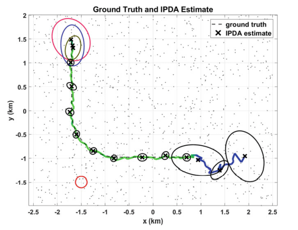
A simulated scenario for the IPDA filter is examined in this section. Elements of $\mathcal{X}$ and $Y$ will be represented using boldface text (e.g., $\mathbf{x}$ and $\mathbf{y}$ ) so that they will not be confused with their 2D spatial components $x$ and $y$. All spatial units are in meters, and all time units are in seconds.
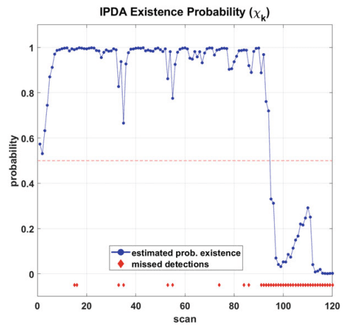
The spatial region of interest is $\mathcal{R}=[-2500.2500] \times[-2500.2500] \subset \mathbb{R}^2$. A point object moves in continuous time through $\mathcal{R}$ at a constant speed of $50 \mathrm{~m} / \mathrm{s}$. Its state space $\mathcal{X} \subset \mathbb{R}^4$ comprises position and velocity components; an element $\mathbf{x} \in X$ is repat time $t_0=0$. It moves at this velocity for $30 \mathrm{~s}$, turns at $3^{\circ}$ per second for the next $30 \mathrm{~s}$, moves in the positive $x$ direction for $30 \mathrm{~s}$, and then “disappears” at time $90 \mathrm{~s}$ with last $x-y$ position of approximately $(700-1000)^T$. From a simulation point of view, this means simply that the object no longer produces sensor measurements.
A sensor provides spatial $x-y$ measurements at $1 \mathrm{~s}$ intervals starting at time $t_1=1$ and ending at time $t_K \equiv t_{120}=120$; that is, $\Delta t=1$. The measurement space $y$ is a subset of $\mathbb{R}^2$, and an element $\mathbf{y} \in Y$ is represented by the $2 \mathrm{D}$ spatial vector $\mathbf{y}=(x y)^T$. At each scan time $t_k$, the object is in state $\mathbf{x}_k \in \mathcal{X}$, and it induces a sensor measurement $\mathbf{y}_k \in \mathcal{Y}$ with probability $p_d=0.9$. Given that the object is detected, a measurement $\mathbf{y}_k$ is generated according to the linear-Gaussian PDF $p_k\left(\mathbf{y}_k \mid \mathbf{x}_k\right)=$ $\mathcal{N}\left(\mathbf{y}_k ; H \mathbf{x}_k, R\right)$, where
$$
H_k \equiv H=\left(\begin{array}{llll}
1 & 0 & 0 & 0 \
0 & 0 & 1 & 0
\end{array}\right) \text { and } R_k \equiv R=\sigma_M^2\left(\begin{array}{ll}
1 & 0 \
0 & 1
\end{array}\right)
$$
with $o_M=40$. In the simulation, no measurement fell outside the region $\mathcal{R}$.
Simulated clutter measurements are realizations of a homogeneous PPP with uniform clutter intensity over $\mathcal{R}$. Specifically, the mean number of clutter measurements $\lambda_k^c \equiv \lambda^c=225$ is constant over all scans, and the clutter $\operatorname{PDF} p_k^c(\mathbf{y}) \equiv \frac{1}{\operatorname{Vol}(\mathcal{R})}=$ $4 \times 10^{-8}$ for $\mathbf{y} \in \mathcal{R}$. Thus, in each scan, there is an average of approximately $0.4$ clutter measurements in a $3 \sigma_M$ measurement window.
Linear-Gaussian assumptions are adopted for object motion. Equations (2.7)-(2.9) become (2.51) -(2.53), respectively. The prior object state $\mu_0(\cdot)$ at time $t_0$ is assumed to be normally distributed with mean $\hat{x}{0 \mid 0}=\mathbf{x}_0$ and diagonal covariance matrix $P{0 \mid 0}=$ $\operatorname{diag}\left(200^2, 10^2, 200^2, 10^2\right)$. The object motion model is assumed stationary, so that $F_k \equiv F$ and $Q_k \equiv Q$ are constant over all scans, where $$
F=\left(\begin{array}{cccc}
1 & \Delta t & 0 & 0 \
0 & 1 & 0 & 0 \
0 & 0 & 1 & \Delta t \
0 & 0 & 0 & 1
\end{array}\right) \text { and } Q=\sigma_p^2\left(\begin{array}{cccc}
\frac{\Delta t^3}{3} & \frac{\Delta t^2}{2} & 0 & 0 \
\frac{\Delta t^2}{2} & \Delta t & 0 & 0 \
0 & 0 & \frac{\Delta t^3}{3} & \frac{\Delta t^2}{2} \
0 & 0 & \frac{\Delta t^2}{2} & \Delta t
\end{array}\right)
$$
with $\sigma_p=5$. No gating is performed. The IPDA prior probability of existence is set to $\chi_0=0.5$, and the IPDA transition matrix parameters given in (2.35) are set to $\pi_k^0-1$ and $\pi_k^1-0.99$ for $k \geq 1$. Tracking filter parameters $\lambda^c, p_d$, and $\sigma_M$ are matched to those of the simulation.
数学代写|组合学代写Combinatorics代考|Joint Probabilistic Data Association (JPDA) Filter
The JPDA filter is a classical Bayesian multiobject estimator that determines the posterior joint PDF on the Cartesian product of the object state spaces, conditioned on all the available measurements. It is impractical for many applications because its computational complexity is NP-hard, which means that runtime grows exponentially with the number of objects and measurements regardless of how the filter is implemented. The JPDA filter is described in many places. The early papers $[2-4]$ lay the foundation, but [5] is more commonly cited as it provides practical application tips and applies JPDA to a passive sonar tracking problem. On the other hand, [6] presents the first $\mathrm{AC}$ derivation of JPDA, and [7] provides more discussion on the AC-JPDA connection.
The JPDA filter is designed for $N \geq 1$ objects. Objects are assumed independent of each other and causally independent of the measurement process. Each object generates at most one measurement in any given scan, and all object measurements are in the space $y$. Measurements are unlabeled, i.e., which object generated which measurement is unknown. Measurements are assigned to at most one object, and the measurement likelihood function depends only on the object to which it is assigned. Measurements not assigned to an object are assigned to a clutter process.
The PDA notation is adjusted to accommodate $N$ objects. The state space of object $n$ is denoted by $\mathcal{X}^n, n=1, \ldots, N$. In many discussions, the object state spaces are taken to be identical, i.e., $\mathcal{X}^n \equiv X$; however, the restriction is unnecessary. The state space for the $N$ objects is the Cartesian product $\chi^1 \times \cdots \times \chi^N$. The a priori PDF at scan $k$ is specified as the product $\mu_{k-1}^1(\cdot) \cdots \mu_{k-1}^N(\cdot)$, where $\mu_{k-1}^n(\cdot)$ is the a priori PDF of object $n$ on $\mathcal{X}^n$.
A superscript $n$ is added to already named PDA functions to indicate that they depend on the object. Thus, for object $n$ at scan $k$, the predicted PDF for object state $x \in \mathcal{X}^n$ is $\mu_k^{n-}(x)$, the probability of object detection is $P d_k^n(x)$, the Markov transition function is $p_k^n(x \mid \cdot)$, the conditional probability of $y \in \mathcal{Y}$ is $p_k^n(y \mid x)$, and the predicted measurement PDF is $\rho_k^n(y)$. Distinct object-induced measurements are mutually independent given an object-measurement assignment and the corresponding object states. Let $\left{y_1, \ldots, y_M\right}, M \geq 1$, represent a collection of measurements, and let $\left(x^1, \ldots, x^N\right)$ represent the object states at scan $k$.
组合学代考
数学代写|组合学代写Combinatorics代考|数值示例:IPDA
本节将研究IPDA滤波器的模拟场景。$\mathcal{X}$和$Y$的元素将使用粗体文本表示(例如,$\mathbf{x}$和$\mathbf{y}$),这样它们就不会与它们的2D空间组件$x$和$y$混淆。 .所有空间单位均为米,所有时间单位均为秒
我们感兴趣的空间区域是$\mathcal{R}=[-2500.2500] \times[-2500.2500] \subset \mathbb{R}^2$。一个点对象以$50 \mathrm{~m} / \mathrm{s}$的恒定速度在连续时间内通过$\mathcal{R}$。其状态空间$\mathcal{X} \subset \mathbb{R}^4$由位置和速度分量组成;元素$\mathbf{x} \in X$是重复时间$t_0=0$。它以这个速度移动到$30 \mathrm{~s}$,以$3^{\circ}$ /秒的速度转动到下一个$30 \mathrm{~s}$,朝着正向$x$的方向移动到$30 \mathrm{~s}$,然后在$90 \mathrm{~s}$时刻“消失”,最后的$x-y$位置大约为$(700-1000)^T$。从模拟的角度来看,这仅仅意味着对象不再产生传感器测量。
传感器以$1 \mathrm{~s}$的间隔提供空间$x-y$测量,从时间$t_1=1$开始到时间$t_K \equiv t_{120}=120$结束;网址是$\Delta t=1$。度量空间$y$是$\mathbb{R}^2$的一个子集,元素$\mathbf{y} \in Y$由$2 \mathrm{D}$空间向量$\mathbf{y}=(x y)^T$表示。在每次扫描时间$t_k$时,对象的状态为$\mathbf{x}_k \in \mathcal{X}$,它诱导一个传感器测量$\mathbf{y}_k \in \mathcal{Y}$,概率为$p_d=0.9$。假设检测到对象,根据线性-高斯PDF $p_k\left(\mathbf{y}_k \mid \mathbf{x}_k\right)=$$\mathcal{N}\left(\mathbf{y}_k ; H \mathbf{x}_k, R\right)$生成一个测量值$\mathbf{y}_k$,其中
$$
H_k \equiv H=\left(\begin{array}{llll}
1 & 0 & 0 & 0 \
0 & 0 & 1 & 0
\end{array}\right) \text { and } R_k \equiv R=\sigma_M^2\left(\begin{array}{ll}
1 & 0 \
0 & 1
\end{array}\right)
$$
with $o_M=40$。在模拟中,没有测量落在$\mathcal{R}$区域之外。
模拟杂波测量是在$\mathcal{R}$上具有均匀杂波强度的均匀PPP的实现。具体地说,杂波测量的平均数$\lambda_k^c \equiv \lambda^c=225$在所有扫描中是恒定的,而杂波为$\mathbf{y} \in \mathcal{R}$的$\operatorname{PDF} p_k^c(\mathbf{y}) \equiv \frac{1}{\operatorname{Vol}(\mathcal{R})}=$$4 \times 10^{-8}$。因此,在每次扫描中,$3 \sigma_M$测量窗口中大约有$0.4$个杂波测量值的平均值 物体运动采用线性-高斯假设。式(2.7)-(2.9)分别变成(2.51)-(2.53)。假设先验对象状态$\mu_0(\cdot)$在$t_0$时刻为正态分布,均值为$\hat{x}{0 \mid 0}=\mathbf{x}_0$,对角协方差矩阵为$P{0 \mid 0}=$$\operatorname{diag}\left(200^2, 10^2, 200^2, 10^2\right)$。假设对象运动模型是平稳的,因此$F_k \equiv F$和$Q_k \equiv Q$在所有扫描中都是常数,其中$$
F=\left(\begin{array}{cccc}
1 & \Delta t & 0 & 0 \
0 & 1 & 0 & 0 \
0 & 0 & 1 & \Delta t \
0 & 0 & 0 & 1
\end{array}\right) \text { and } Q=\sigma_p^2\left(\begin{array}{cccc}
\frac{\Delta t^3}{3} & \frac{\Delta t^2}{2} & 0 & 0 \
\frac{\Delta t^2}{2} & \Delta t & 0 & 0 \
0 & 0 & \frac{\Delta t^3}{3} & \frac{\Delta t^2}{2} \
0 & 0 & \frac{\Delta t^2}{2} & \Delta t
\end{array}\right)
$$
和$\sigma_p=5$。不执行门控。IPDA存在先验概率设为$\chi_0=0.5$,(2.35)中给出的IPDA转换矩阵参数设为$\pi_k^0-1$,对于$k \geq 1$设为$\pi_k^1-0.99$。跟踪过滤器参数$\lambda^c, p_d$、$\sigma_M$与仿真匹配。
.
数学代写|组合学代写Combinatorics代考|联合概率数据关联(JPDA)过滤器
.
JPDA滤波器是一个经典的贝叶斯多目标估计器,它在所有可用的测量条件下,确定物体状态空间笛卡尔积上的后关节PDF。对于许多应用程序来说,它是不切实际的,因为它的计算复杂度是NP-hard,这意味着运行时随着对象和度量的数量呈指数增长,而不管过滤器是如何实现的。JPDA过滤器在很多地方都有描述。早期的论文$[2-4]$奠定了基础,但[5]更常被引用,因为它提供了实际的应用技巧,并将JPDA应用于被动声纳跟踪问题。另一方面,[6]给出了JPDA的第一个$\mathrm{AC}$派生,[7]提供了关于AC-JPDA连接的更多讨论
JPDA过滤器是为$N \geq 1$对象设计的。假设对象彼此独立,并且在因果上独立于测量过程。在任何给定的扫描中,每个对象最多生成一个测量值,所有对象测量值都位于空间$y$中。测量是未标记的,即,哪个对象生成哪个测量是未知的。测量值被分配给最多一个对象,测量似然函数只依赖于被分配的对象。没有分配给对象的度量值被分配给杂波进程
PDA符号被调整为适应$N$对象。对象$n$的状态空间由$\mathcal{X}^n, n=1, \ldots, N$表示。在许多讨论中,对象状态空间被认为是相同的,即$\mathcal{X}^n \equiv X$;然而,这种限制是不必要的。$N$对象的状态空间是$\chi^1 \times \cdots \times \chi^N$的笛卡尔积。扫描$k$上的先验PDF被指定为产品$\mu_{k-1}^1(\cdot) \cdots \mu_{k-1}^N(\cdot)$,其中$\mu_{k-1}^n(\cdot)$是$\mathcal{X}^n$上的对象$n$的先验PDF 在已经命名的PDA函数中添加上标$n$,以指示它们依赖于对象。因此,对于扫描位置为$k$的目标$n$,目标状态$x \in \mathcal{X}^n$的预测PDF为$\mu_k^{n-}(x)$,目标检测概率为$P d_k^n(x)$,马尔可夫过渡函数为$p_k^n(x \mid \cdot)$, $y \in \mathcal{Y}$的条件概率为$p_k^n(y \mid x)$,预测测量PDF为$\rho_k^n(y)$。给定一个对象测量分配和相应的对象状态,不同的对象诱导测量是相互独立的。设$\left{y_1, \ldots, y_M\right}, M \geq 1$表示测量的集合,设$\left(x^1, \ldots, x^N\right)$表示扫描$k$时的对象状态。

统计代写请认准statistics-lab™. statistics-lab™为您的留学生涯保驾护航。
金融工程代写
金融工程是使用数学技术来解决金融问题。金融工程使用计算机科学、统计学、经济学和应用数学领域的工具和知识来解决当前的金融问题,以及设计新的和创新的金融产品。
非参数统计代写
非参数统计指的是一种统计方法,其中不假设数据来自于由少数参数决定的规定模型;这种模型的例子包括正态分布模型和线性回归模型。
广义线性模型代考
广义线性模型(GLM)归属统计学领域,是一种应用灵活的线性回归模型。该模型允许因变量的偏差分布有除了正态分布之外的其它分布。
术语 广义线性模型(GLM)通常是指给定连续和/或分类预测因素的连续响应变量的常规线性回归模型。它包括多元线性回归,以及方差分析和方差分析(仅含固定效应)。
有限元方法代写
有限元方法(FEM)是一种流行的方法,用于数值解决工程和数学建模中出现的微分方程。典型的问题领域包括结构分析、传热、流体流动、质量运输和电磁势等传统领域。
有限元是一种通用的数值方法,用于解决两个或三个空间变量的偏微分方程(即一些边界值问题)。为了解决一个问题,有限元将一个大系统细分为更小、更简单的部分,称为有限元。这是通过在空间维度上的特定空间离散化来实现的,它是通过构建对象的网格来实现的:用于求解的数值域,它有有限数量的点。边界值问题的有限元方法表述最终导致一个代数方程组。该方法在域上对未知函数进行逼近。[1] 然后将模拟这些有限元的简单方程组合成一个更大的方程系统,以模拟整个问题。然后,有限元通过变化微积分使相关的误差函数最小化来逼近一个解决方案。
tatistics-lab作为专业的留学生服务机构,多年来已为美国、英国、加拿大、澳洲等留学热门地的学生提供专业的学术服务,包括但不限于Essay代写,Assignment代写,Dissertation代写,Report代写,小组作业代写,Proposal代写,Paper代写,Presentation代写,计算机作业代写,论文修改和润色,网课代做,exam代考等等。写作范围涵盖高中,本科,研究生等海外留学全阶段,辐射金融,经济学,会计学,审计学,管理学等全球99%专业科目。写作团队既有专业英语母语作者,也有海外名校硕博留学生,每位写作老师都拥有过硬的语言能力,专业的学科背景和学术写作经验。我们承诺100%原创,100%专业,100%准时,100%满意。
随机分析代写
随机微积分是数学的一个分支,对随机过程进行操作。它允许为随机过程的积分定义一个关于随机过程的一致的积分理论。这个领域是由日本数学家伊藤清在第二次世界大战期间创建并开始的。
时间序列分析代写
随机过程,是依赖于参数的一组随机变量的全体,参数通常是时间。 随机变量是随机现象的数量表现,其时间序列是一组按照时间发生先后顺序进行排列的数据点序列。通常一组时间序列的时间间隔为一恒定值(如1秒,5分钟,12小时,7天,1年),因此时间序列可以作为离散时间数据进行分析处理。研究时间序列数据的意义在于现实中,往往需要研究某个事物其随时间发展变化的规律。这就需要通过研究该事物过去发展的历史记录,以得到其自身发展的规律。
回归分析代写
多元回归分析渐进(Multiple Regression Analysis Asymptotics)属于计量经济学领域,主要是一种数学上的统计分析方法,可以分析复杂情况下各影响因素的数学关系,在自然科学、社会和经济学等多个领域内应用广泛。
MATLAB代写
MATLAB 是一种用于技术计算的高性能语言。它将计算、可视化和编程集成在一个易于使用的环境中,其中问题和解决方案以熟悉的数学符号表示。典型用途包括:数学和计算算法开发建模、仿真和原型制作数据分析、探索和可视化科学和工程图形应用程序开发,包括图形用户界面构建MATLAB 是一个交互式系统,其基本数据元素是一个不需要维度的数组。这使您可以解决许多技术计算问题,尤其是那些具有矩阵和向量公式的问题,而只需用 C 或 Fortran 等标量非交互式语言编写程序所需的时间的一小部分。MATLAB 名称代表矩阵实验室。MATLAB 最初的编写目的是提供对由 LINPACK 和 EISPACK 项目开发的矩阵软件的轻松访问,这两个项目共同代表了矩阵计算软件的最新技术。MATLAB 经过多年的发展,得到了许多用户的投入。在大学环境中,它是数学、工程和科学入门和高级课程的标准教学工具。在工业领域,MATLAB 是高效研究、开发和分析的首选工具。MATLAB 具有一系列称为工具箱的特定于应用程序的解决方案。对于大多数 MATLAB 用户来说非常重要,工具箱允许您学习和应用专业技术。工具箱是 MATLAB 函数(M 文件)的综合集合,可扩展 MATLAB 环境以解决特定类别的问题。可用工具箱的领域包括信号处理、控制系统、神经网络、模糊逻辑、小波、仿真等。