如果你也在 怎样代写有限元方法finite differences method 这个学科遇到相关的难题,请随时右上角联系我们的24/7代写客服。有限元方法finite differences method领域中所有的物理系统都可以用边界/初值问题来表示。在这本书中,我们主要集中在解决一维和二维线性弹性和传热问题。将这些解决方案技术扩展到三维分析是直接的,因此为了保持表示的清晰性并避免重复,这里不进行讨论。
有限元方法finite differences method提供了一种系统的方法来推导简单子区域的近似函数,通过这些近似函数可以表示几何上复杂的区域。在有限元法中,近似函数是分段多项式(即只在子区域上定义的多项式,称为单元)。
statistics-lab™ 为您的留学生涯保驾护航 在代写有限元方法Finite Element Method方面已经树立了自己的口碑, 保证靠谱, 高质且原创的统计Statistics代写服务。我们的专家在代写有限元方法Finite Element Method代写方面经验极为丰富,各种代写有限元方法Finite Element Method相关的作业也就用不着说。

数学代写|有限元方法代写Finite Element Method代考|Preliminary Comments
Numerical evaluation of integrals, called numerical integration or numerical quadrature, involves approximation of the integrand by a polynomial of sufficient degree, because the integral of a polynomial can be evaluated exactly. The integrals are generally expressed in terms of the coordinate appearing in the problem description (like $x$ or $r$ ). We shall call $x$ and $r$ as the problem coordinates or global coordinates. Since the finite element approximation (or interpolation) functions are derived over an element, it is convenient to use a local (i.e., element) coordinate, such as $\bar{x}$ used earlier.
For example, consider the integral,
$$
I_e=\int_{x_a^e}^{x_b^e} F_e(x) d x=\int_0^{h_e} F^e(\bar{x}) d \bar{x}
$$
where $F^e$ is a function of $x=x_a^e+\bar{x}$, and $h_e=x_b^e-x_a^e$. We approximate the function $F^e(\bar{x})$ in $\Omega^e$ by a polynomial
$$
F^e(\bar{x}) \approx \sum_{I=1}^N F_I^e \psi_I^e(\bar{x})
$$
where $F_I^e$ denotes the value of $F^e(\bar{x})$ at the $I$ th point $\bar{x}_I$ of the interval $\left[0, h_e\right]$ and $\psi_I^e(\bar{x})$ are polynomials of degree $N-1$ in the interval. The representation can be viewed as the finite element interpolation of $F^e(\bar{x})$, where $F_I^e$ is the value of the function at the Ith node. The interpolation functions $\psi_I^e(\bar{x})$ can be of the Lagrange type or the Hermite type.
Substitution of Eq. (8.2.2) into Eq. (8.2.1) and evaluation of the integral give an approximate value of the integral $I_e$. For example, suppose that we choose linear interpolation of $F^e(\bar{x})$, as shown in Fig. 8.2.1. For $N=2$, we have
$$
\psi_1^e=1-\frac{\bar{x}}{h_e}, \quad \psi_2^e=\frac{\bar{x}}{h_e}, \quad \int_0^{h_e} \psi_I^e(\bar{x}) d \bar{x}=\frac{h_e}{2} \quad(I=1,2)
$$
and
$$
I_e=\frac{h_e}{2}\left(F_1^e+F_2^e\right), \quad F_1^e=F^e(0), \quad F_2^e=F^e\left(h_e\right)
$$
Thus, the value of the integral is given by the area of a trapezoid used to approximate the area under the function $F^e(\bar{x})$ (see Fig. 8.2.1). Equation (8.2.3b) is known as the trapezoidal rule of numerical integration.
数学代写|有限元方法代写Finite Element Method代考|Natural Coordinates
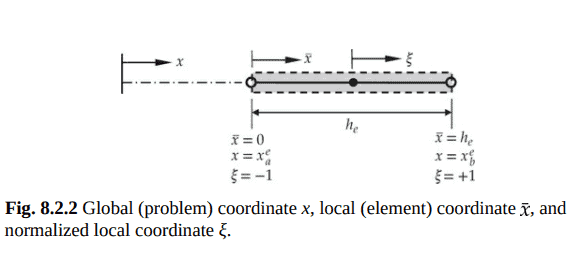
Of all the quadrature formulae, the Gauss-Legendre quadrature is the most commonly used. The details of the method itself will be discussed shortly. The quadrature formula requires the integral to be cast as one to be evaluated over the interval (element) $\hat{\bar{\Omega}}^e \equiv[-1,1}$ This requires the transformation of the problem coordinate $x$ (i.e., the coordinate used to describe the governing equation) to the element coordinate $\xi$ such that the integrals are posed on [-1, 1] (see Fig. 8.2.2). Thus, the relationship between $x$ and $\xi$ is linear and it can be established with the help of the conditions
when $x=x_a^e, \quad \xi=-1 ;$ and when $x=x_b^e, \quad \xi=1$
This transformation between $x$ and $\xi$ can be represented by the linear “stretch” mapping
$$
x=a^e+b^e \xi \text { for } x \text { in } \bar{\Omega}^e=\left[x_a^e, x_b^e\right]
$$
where $a^e$ and $b^e$ are constants to be determined such that conditions in Eq. (8.2.6a) hold:
$$
x_a^e=a^e+b^e \cdot(-1), \quad x_b^e=a^e+b^e .
$$
Solving for $a^e$ and $b^e$, we obtain
$$
b^e=\frac{1}{2}\left(x_b^e-x_a^e\right)=\frac{1}{2} h_e, \quad a^e=\frac{1}{2}\left(x_b^e+x_a^e\right)=x_a^e+\frac{1}{2} h_e
$$
Hence the transformation between $x$ and $\xi$ becomes
$$
x(\xi)=\frac{1}{2}\left(x_b^e+x_a^e\right)+\frac{1}{2}\left(x_b^e-x_a^e\right) \xi=x_a^e \frac{1}{2}(1-\xi) x_b^e \frac{1}{2}(1+\xi)=x_a^e+\frac{1}{2} h_e(1+\xi)
$$
where $x_a^e$ and $x_b^e$ denote the global coordinates of the left end and the right end, respectively, of the element $\bar{\Omega}^e$ and $h_e$ is the element length (see Fig. 8.2.2).
The local coordinate $\xi$ is called the normal coordinate or natural coordinate, and its values always lie between -1 and 1 , with its origin at the center of the 1-D element. The local coordinate $\xi$ is useful in two ways: it is (1) convenient in constructing the interpolation functions and (2) required in the numerical integration based on the Gauss-Legendre quadrature.
The derivation of the Lagrange family of interpolation functions in terms of the natural coordinate $\xi$ is made easy by the following interpolation property of the approximation functions:
$$
\psi_i^e\left(\xi_j\right)= \begin{cases}1 & \text { if } i=j \ 0 & \text { if } i \neq j\end{cases}
$$
where $\xi_j$ is the $\xi$-coordinate of the $j$ th node in the element. For an element with $n$ nodes, the Lagrange interpolation functions $\psi_i^e(i=1,2, \ldots, n)$ are polynomials of degree $n-1$. To construct $\psi_i^e$ satisfying the properties in Eq. (8.2.8), we proceed as follows. For each $\psi_i^e$, we form the product of $n-1$ linear functions $\xi-\xi_j(j=1,2, \ldots, i-1, i+1, \ldots, n$ and $j \neq i)$ :
$$
\psi_i^e=c_i\left(\xi-\xi_1\right)\left(\xi-\xi_2\right) \cdots\left(\xi-\xi_{i-1}\right)\left(\xi-\xi_{i+1}\right) \cdots\left(\xi-\xi_n\right)
$$
Note that $\psi_i^e$ is zero at all nodes except the $i$ th. Next we determine the constant $c_i$ such that $\psi_i^e=1$ at $\xi-\xi_i$ :
$$
c_i=\left[\left(\xi_i-\xi_1\right)\left(\xi_i-\xi_2\right) \cdots\left(\xi_i-\xi_{i-1}\right)\left(\xi_i-\xi_{i+1}\right) \cdots\left(\xi_i-\xi_n\right)\right]^{-1}
$$
Thus, the interpolation function associated with node $i$ is
$$
\psi_i^e(\xi)=\frac{\left(\xi-\xi_1\right)\left(\xi-\xi_2\right) \cdots\left(\xi-\xi_{i-1}\right)\left(\xi-\xi_{i+1}\right) \cdots\left(\xi-\xi_n\right)}{\left(\xi_i-\xi_1\right)\left(\xi_i-\xi_2\right) \cdots\left(\xi_i-\xi_{i-1}\right)\left(\xi_i-\xi_{i+1}\right) \cdots\left(\xi_i-\xi_n\right)}
$$

有限元方法代考
数学代写|有限元方法代写Finite Element Method代考|Preliminary Comments
积分的数值计算,称为数值积分或数值正交,涉及到用一个充分次多项式逼近被积函数,因为多项式的积分可以精确地求值。积分通常用问题描述(如$x$或$r$)中出现的坐标来表示。我们称$x$和$r$为问题坐标或全局坐标。由于有限元逼近(或插值)函数是在一个元素上导出的,因此使用局部(即元素)坐标很方便,例如前面使用的$\bar{x}$。
例如,考虑积分,
$$
I_e=\int_{x_a^e}^{x_b^e} F_e(x) d x=\int_0^{h_e} F^e(\bar{x}) d \bar{x}
$$
其中$F^e$是$x=x_a^e+\bar{x}$的函数,$h_e=x_b^e-x_a^e$。我们用多项式近似$\Omega^e$中的$F^e(\bar{x})$函数
$$
F^e(\bar{x}) \approx \sum_{I=1}^N F_I^e \psi_I^e(\bar{x})
$$
式中$F_I^e$为区间$I$第th点$\bar{x}_I$处$F^e(\bar{x})$的值$\left[0, h_e\right]$, $\psi_I^e(\bar{x})$为区间内$N-1$次多项式。表示可以看作是$F^e(\bar{x})$的有限元插值,其中$F_I^e$是函数在第i个节点处的值。插值函数$\psi_I^e(\bar{x})$可以是拉格朗日类型或埃尔米特类型。
将Eq.(8.2.2)代入Eq.(8.2.1)并对积分进行计算,得到积分$I_e$的近似值。例如,假设我们选择$F^e(\bar{x})$线性插值,如图8.2.1所示。对于$N=2$,我们有
$$
\psi_1^e=1-\frac{\bar{x}}{h_e}, \quad \psi_2^e=\frac{\bar{x}}{h_e}, \quad \int_0^{h_e} \psi_I^e(\bar{x}) d \bar{x}=\frac{h_e}{2} \quad(I=1,2)
$$
和
$$
I_e=\frac{h_e}{2}\left(F_1^e+F_2^e\right), \quad F_1^e=F^e(0), \quad F_2^e=F^e\left(h_e\right)
$$
因此,积分的值由用于近似函数$F^e(\bar{x})$下的面积的梯形面积给出(见图8.2.1)。式(8.2.3b)称为数值积分的梯形法则。
数学代写|有限元方法代写Finite Element Method代考|Natural Coordinates
在所有的正交公式中,高斯-勒让德正交是最常用的。稍后将讨论该方法本身的细节。积分公式要求将积分转换为一个在区间(元素)$\hat{\bar{\Omega}}^e \equiv[-1,1}$上求值的积分,这需要将问题坐标$x$(即,用于描述控制方程的坐标)转换为元素坐标$\xi$,以便将积分置于[- 1,1]上(见图8.2.2)。因此,$x$与$\xi$之间的关系是线性的,可以借助条件来建立
当$x=x_a^e, \quad \xi=-1 ;$和当$x=x_b^e, \quad \xi=1$
$x$和$\xi$之间的转换可以用线性“拉伸”映射表示
$$
x=a^e+b^e \xi \text { for } x \text { in } \bar{\Omega}^e=\left[x_a^e, x_b^e\right]
$$
其中$a^e$和$b^e$为待确定的常数,使式(8.2.6a)中的条件成立:
$$
x_a^e=a^e+b^e \cdot(-1), \quad x_b^e=a^e+b^e .
$$
求解$a^e$和$b^e$,得到
$$
b^e=\frac{1}{2}\left(x_b^e-x_a^e\right)=\frac{1}{2} h_e, \quad a^e=\frac{1}{2}\left(x_b^e+x_a^e\right)=x_a^e+\frac{1}{2} h_e
$$
因此$x$和$\xi$之间的转换变成
$$
x(\xi)=\frac{1}{2}\left(x_b^e+x_a^e\right)+\frac{1}{2}\left(x_b^e-x_a^e\right) \xi=x_a^e \frac{1}{2}(1-\xi) x_b^e \frac{1}{2}(1+\xi)=x_a^e+\frac{1}{2} h_e(1+\xi)
$$
其中$x_a^e$和$x_b^e$分别为元素左端和右端的全局坐标,$\bar{\Omega}^e$和$h_e$为元素长度(见图8.2.2)。
局部坐标$\xi$称为法坐标或自然坐标,其值始终在-1到1之间,原点位于一维元素的中心。局部坐标$\xi$在两个方面是有用的:(1)在构造插值函数时是方便的;(2)在基于高斯-勒让德正交的数值积分中是必需的。
用自然坐标$\xi$来推导拉格朗日插值函数族是很容易的,因为近似函数的以下插值性质:
$$
\psi_i^e\left(\xi_j\right)= \begin{cases}1 & \text { if } i=j \ 0 & \text { if } i \neq j\end{cases}
$$
其中$\xi_j$是元素中$j$节点的$\xi$ -坐标。对于具有$n$节点的元素,拉格朗日插值函数$\psi_i^e(i=1,2, \ldots, n)$是次多项式$n-1$。为了构造满足式(8.2.8)中的性质的$\psi_i^e$,我们进行如下操作。对于每个$\psi_i^e$,我们形成$n-1$线性函数$\xi-\xi_j(j=1,2, \ldots, i-1, i+1, \ldots, n$与$j \neq i)$的乘积:
$$
\psi_i^e=c_i\left(\xi-\xi_1\right)\left(\xi-\xi_2\right) \cdots\left(\xi-\xi_{i-1}\right)\left(\xi-\xi_{i+1}\right) \cdots\left(\xi-\xi_n\right)
$$
注意,除了第$i$个节点外,$\psi_i^e$在所有节点上都为零。接下来,我们确定常数$c_i$,使$\psi_i^e=1$ at $\xi-\xi_i$:
$$
c_i=\left[\left(\xi_i-\xi_1\right)\left(\xi_i-\xi_2\right) \cdots\left(\xi_i-\xi_{i-1}\right)\left(\xi_i-\xi_{i+1}\right) \cdots\left(\xi_i-\xi_n\right)\right]^{-1}
$$
因此,节点$i$对应的插值函数为
$$
\psi_i^e(\xi)=\frac{\left(\xi-\xi_1\right)\left(\xi-\xi_2\right) \cdots\left(\xi-\xi_{i-1}\right)\left(\xi-\xi_{i+1}\right) \cdots\left(\xi-\xi_n\right)}{\left(\xi_i-\xi_1\right)\left(\xi_i-\xi_2\right) \cdots\left(\xi_i-\xi_{i-1}\right)\left(\xi_i-\xi_{i+1}\right) \cdots\left(\xi_i-\xi_n\right)}
$$

统计代写请认准statistics-lab™. statistics-lab™为您的留学生涯保驾护航。
金融工程代写
金融工程是使用数学技术来解决金融问题。金融工程使用计算机科学、统计学、经济学和应用数学领域的工具和知识来解决当前的金融问题,以及设计新的和创新的金融产品。
非参数统计代写
非参数统计指的是一种统计方法,其中不假设数据来自于由少数参数决定的规定模型;这种模型的例子包括正态分布模型和线性回归模型。
广义线性模型代考
广义线性模型(GLM)归属统计学领域,是一种应用灵活的线性回归模型。该模型允许因变量的偏差分布有除了正态分布之外的其它分布。
术语 广义线性模型(GLM)通常是指给定连续和/或分类预测因素的连续响应变量的常规线性回归模型。它包括多元线性回归,以及方差分析和方差分析(仅含固定效应)。
有限元方法代写
有限元方法(FEM)是一种流行的方法,用于数值解决工程和数学建模中出现的微分方程。典型的问题领域包括结构分析、传热、流体流动、质量运输和电磁势等传统领域。
有限元是一种通用的数值方法,用于解决两个或三个空间变量的偏微分方程(即一些边界值问题)。为了解决一个问题,有限元将一个大系统细分为更小、更简单的部分,称为有限元。这是通过在空间维度上的特定空间离散化来实现的,它是通过构建对象的网格来实现的:用于求解的数值域,它有有限数量的点。边界值问题的有限元方法表述最终导致一个代数方程组。该方法在域上对未知函数进行逼近。[1] 然后将模拟这些有限元的简单方程组合成一个更大的方程系统,以模拟整个问题。然后,有限元通过变化微积分使相关的误差函数最小化来逼近一个解决方案。
tatistics-lab作为专业的留学生服务机构,多年来已为美国、英国、加拿大、澳洲等留学热门地的学生提供专业的学术服务,包括但不限于Essay代写,Assignment代写,Dissertation代写,Report代写,小组作业代写,Proposal代写,Paper代写,Presentation代写,计算机作业代写,论文修改和润色,网课代做,exam代考等等。写作范围涵盖高中,本科,研究生等海外留学全阶段,辐射金融,经济学,会计学,审计学,管理学等全球99%专业科目。写作团队既有专业英语母语作者,也有海外名校硕博留学生,每位写作老师都拥有过硬的语言能力,专业的学科背景和学术写作经验。我们承诺100%原创,100%专业,100%准时,100%满意。
随机分析代写
随机微积分是数学的一个分支,对随机过程进行操作。它允许为随机过程的积分定义一个关于随机过程的一致的积分理论。这个领域是由日本数学家伊藤清在第二次世界大战期间创建并开始的。
时间序列分析代写
随机过程,是依赖于参数的一组随机变量的全体,参数通常是时间。 随机变量是随机现象的数量表现,其时间序列是一组按照时间发生先后顺序进行排列的数据点序列。通常一组时间序列的时间间隔为一恒定值(如1秒,5分钟,12小时,7天,1年),因此时间序列可以作为离散时间数据进行分析处理。研究时间序列数据的意义在于现实中,往往需要研究某个事物其随时间发展变化的规律。这就需要通过研究该事物过去发展的历史记录,以得到其自身发展的规律。
回归分析代写
多元回归分析渐进(Multiple Regression Analysis Asymptotics)属于计量经济学领域,主要是一种数学上的统计分析方法,可以分析复杂情况下各影响因素的数学关系,在自然科学、社会和经济学等多个领域内应用广泛。
MATLAB代写
MATLAB 是一种用于技术计算的高性能语言。它将计算、可视化和编程集成在一个易于使用的环境中,其中问题和解决方案以熟悉的数学符号表示。典型用途包括:数学和计算算法开发建模、仿真和原型制作数据分析、探索和可视化科学和工程图形应用程序开发,包括图形用户界面构建MATLAB 是一个交互式系统,其基本数据元素是一个不需要维度的数组。这使您可以解决许多技术计算问题,尤其是那些具有矩阵和向量公式的问题,而只需用 C 或 Fortran 等标量非交互式语言编写程序所需的时间的一小部分。MATLAB 名称代表矩阵实验室。MATLAB 最初的编写目的是提供对由 LINPACK 和 EISPACK 项目开发的矩阵软件的轻松访问,这两个项目共同代表了矩阵计算软件的最新技术。MATLAB 经过多年的发展,得到了许多用户的投入。在大学环境中,它是数学、工程和科学入门和高级课程的标准教学工具。在工业领域,MATLAB 是高效研究、开发和分析的首选工具。MATLAB 具有一系列称为工具箱的特定于应用程序的解决方案。对于大多数 MATLAB 用户来说非常重要,工具箱允许您学习和应用专业技术。工具箱是 MATLAB 函数(M 文件)的综合集合,可扩展 MATLAB 环境以解决特定类别的问题。可用工具箱的领域包括信号处理、控制系统、神经网络、模糊逻辑、小波、仿真等。