如果你也在 怎样代写线性回归Linear Regression 这个学科遇到相关的难题,请随时右上角联系我们的24/7代写客服。线性回归Linear Regression在统计学中,是对标量响应和一个或多个解释变量(也称为因变量和自变量)之间的关系进行建模的一种线性方法。一个解释变量的情况被称为简单线性回归;对于一个以上的解释变量,这一过程被称为多元线性回归。这一术语不同于多元线性回归,在多元线性回归中,预测的是多个相关的因变量,而不是一个标量变量。
线性回归Linear Regression在线性回归中,关系是用线性预测函数建模的,其未知的模型参数是根据数据估计的。最常见的是,假设给定解释变量(或预测因子)值的响应的条件平均值是这些值的仿生函数;不太常见的是,使用条件中位数或其他一些量化指标。像所有形式的回归分析一样,线性回归关注的是给定预测因子值的反应的条件概率分布,而不是所有这些变量的联合概率分布,这是多元分析的领域。
statistics-lab™ 为您的留学生涯保驾护航 在代写线性回归分析linear regression analysis方面已经树立了自己的口碑, 保证靠谱, 高质且原创的统计Statistics代写服务。我们的专家在代写线性回归分析linear regression analysis代写方面经验极为丰富,各种代写线性回归分析linear regression analysis相关的作业也就用不着说。
统计代写|线性回归分析代写linear regression analysis代考|UNDERSTANDING PARAMETER ESTIMATES
Parameters in mean functions have units attached to them. For example, the fitted mean function for the fuel consumption data is
$$
\mathrm{E}(\text { Fuel } \mid X)=154.19-4.23 \text { Tax }+0.47 \text { Dic }-6.14 \text { Income }+18.54 \log (\text { Miles })
$$
Fuel is measured in gallons, and so all the quantities on the right of this equation must also be in gallons. The intercept is 154.19 gallons. Since Income is measured in thousands of dollars, the coefficient for Income must be in gallons per thousand dollars of income. Similarly, the units for the coefficient for Tax is gallons per cent of $\operatorname{tax}$.
Rate of Change
The usual interpretation of an estimated coefficient is as a rate of change: increasing Tax rate by one cent should decrease consumption, all other factors being held constant, by about 4.23 gallons per person. This assumes that a predictor can in fact be changed without affecting the other terms in the mean function and that the available data will apply when the predictor is so changed. The fuel data are observational since the assignment of values for the predictors was not under the control of the analyst, so whether increasing taxes would cause a decrease in fuel consumption cannot be assessed from these data. From these data, we can observe association but not cause: states with higher tax rates are observed to have lower fuel consumption. To draw conclusions concerning the effects of changing tax rates, the rates must in fact be changed and the results observed.
The coefficient estimate of $\log ($ Miles) is 18.55 , meaning that a change of one unit in $\log ($ Miles $)$ is associated with an 18.55 gallon per person increase in consumption. States with more roads have higher per capita fuel consumption. Since we used base-two logarithms in this problem, increasing $\log$ (Miles) by one unit means that the value of Miles doubles. If we double the amount of road in a state, we expect to increase fuel consumption by about 18.55 gallons per person. If we had used base-ten logarithms, then the fitted mean function would be
$$
\mathrm{E}(\text { Fuel } \mid X)=154.19-4.23 \text { Tax }+0.47 \text { Dlic }-6.14 \text { Income }+61.61 \log {10}(\text { Miles }) $$ The only change in the fitted model is for the coefficient for the log of Miles, which is now interpreted as a change in expected Fuel consumption when $\log {10}$ (Miles) increases by one unit, or when Miles is multiplied by 10 .
统计代写|线性回归分析代写linear regression analysis代考|Signs of Estimates
The sign of a parameter estimate indicates the direction of the relationship between the term and the response. In multiple regression, if the terms are correlated, the sign of a coefficient may change depending on the other terms in the model. While this is mathematically possible and, occasionally, scientifically reasonable, it certainly makes interpretation more difficult. Sometimes this problem can be removed by redefining the terms into new linear combinations that are easier to interpret.
Interpretation Depends on Other Terms in the Mean Function
The value of a parameter estimate not only depends on the other terms in a mean function but it can also change if the other terms are replaced by linear combinations of the terms.
Berkeley Guidance Study
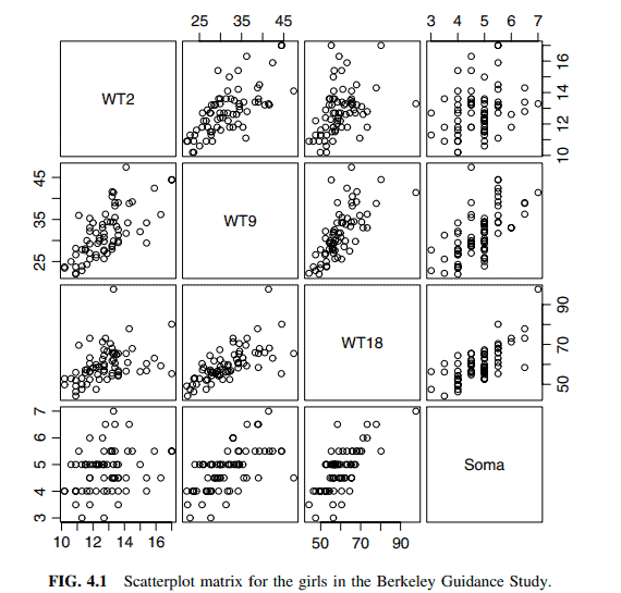
Data from the Berkeley Guidance Study on the growth of boys and girls are given in Problem 3.1. As in Problem 3.1, we will view Soma as the response, but consider the three predictors $W T 2, W T 9, W T 18$ for the $n=70$ girls in the study. The scatterplot matrix for these four variables is given in Figure 4.1. First look at the last row of this figure, giving the marginal response plots of Soma versus each of the three potential predictors. For each of these plots, we see that Soma is increasing with the potential predictor on the average, although the relationship is strongest at the oldest age and weakest at the youngest age. The two-dimensional plots of each pair of predictors suggest that the predictors are correlated among themselves. Taken together, we have evidence that the regression on all three predictors cannot be viewed as just the sum of the three separate simple regressions because we must account for the correlations between the terms.
We will proceed with this example using the three original predictors as terms and Soma as the response. We are encouraged to do this because of the appearance of the scatterplot matrix. Since each of the two-dimensional plots appear to be well summarized by a straight-line mean function, we will see later that this suggests that the regression of the response on the original predictors without transformation is likely to be appropriate.
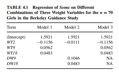
The parameter estimates for the regression of Soma on WT2, WT9, and WT18 given in the column marked “Model 1” in Table 4.1 leads to the unexpected conclusion that heavier girls at age two may tend to be thinner, have lower expected somatotype, at age 18 . We reach this conclusion because the $t$-statistic for testing the coefficient equal to zero, which is not shown in the table, has a significance level of about 0.06 . The sign, and the weak significance, may be due to the correlations between the terms. In place of the preceding variables, consider the following:
$$
\begin{aligned}
W T 2 & =\text { Weight at age } 2 \
D W 9=W T 9-W T 2 & =\text { Weight gain from age } 2 \text { to } 9 \
D W 18=W T 18-W T 9 & =\text { Weight gain from age } 9 \text { to } 18
\end{aligned}
$$

线性回归代写
统计代写|线性回归分析代写linear regression analysis代考|UNDERSTANDING PARAMETER ESTIMATES
平均函数中的参数有附加的单位。例如,油耗数据的拟合均值函数为
$$
\mathrm{E}(\text { Fuel } \mid X)=154.19-4.23 \text { Tax }+0.47 \text { Dic }-6.14 \text { Income }+18.54 \log (\text { Miles })
$$
燃料的单位是加仑,所以等式右边的所有量也必须是加仑。截距是154.19加仑。由于收入是以千美元为单位计算的,因此收入系数必须以每千美元收入的加仑为单位。同样,税收系数的单位是$\operatorname{tax}$的加仑%。
变化率
对估计系数的通常解释是变化率:在所有其他因素保持不变的情况下,税率每增加一美分,人均消费量应减少约4.23加仑。这假设预测器实际上可以改变而不影响平均函数中的其他项,并且当预测器发生这种改变时,可用数据将适用。燃料数据是观察性的,因为预测值的分配不在分析人员的控制之下,因此增加税收是否会导致燃料消耗的减少无法从这些数据中评估。从这些数据中,我们可以观察到关联,但不能观察到原因:观察到税率较高的州燃料消耗较低。为了得出关于税率变化的影响的结论,税率实际上必须改变,结果必须观察到。
$\log ($英里数)的系数估计值为18.55,这意味着$\log ($英里数$)$每变化一个单位,人均消耗就会增加18.55加仑。拥有更多道路的州人均燃料消耗量更高。由于我们在这个问题中使用了以2为底的对数,因此将$\log$(英里)增加一个单位意味着英里的值加倍。如果我们将一个州的道路数量增加一倍,我们预计每人将增加约18.55加仑的燃料消耗。如果我们使用以10为底的对数,那么拟合的均值函数将是
$$
\mathrm{E}(\text { Fuel } \mid X)=154.19-4.23 \text { Tax }+0.47 \text { Dlic }-6.14 \text { Income }+61.61 \log {10}(\text { Miles }) $$拟合模型中唯一的变化是里程对数的系数,当$\log {10}$(里程)增加一个单位或里程乘以10时,它现在被解释为预期燃料消耗的变化。
统计代写|线性回归分析代写linear regression analysis代考|Signs of Estimates
参数估计的符号表示项和响应之间关系的方向。在多元回归中,如果项是相关的,则系数的符号可能会根据模型中的其他项而变化。虽然这在数学上是可能的,有时在科学上也是合理的,但它确实使解释变得更加困难。有时,这个问题可以通过将术语重新定义为更容易解释的新线性组合来解决。
解释取决于平均函数中的其他项
参数估计的值不仅取决于平均函数中的其他项,而且如果其他项被这些项的线性组合所取代,它也会改变。
伯克利导引研究
关于男孩和女孩成长的伯克利指导研究数据在问题3.1中给出。与问题3.1一样,我们将把Soma视为响应,但考虑研究中$n=70$女孩的三个预测因子$W T 2, W T 9, W T 18$。这四个变量的散点图矩阵如图4.1所示。首先看一下这张图的最后一行,给出了Soma相对于三种潜在预测因子的边际响应图。对于每一个图,我们看到Soma随着潜在预测因子的平均增长而增加,尽管这种关系在年龄最大的时候最强,在年龄最小的时候最弱。每对预测因子的二维图表明,预测因子之间是相关的。综上所述,我们有证据表明,所有三个预测因子的回归不能仅仅被视为三个单独的简单回归的总和,因为我们必须考虑到这些项之间的相关性。
我们将使用三个原始预测器作为项并使用Soma作为响应来继续这个示例。我们被鼓励这样做,因为散点图矩阵的出现。由于每个二维图似乎都被一个直线平均函数很好地概括了,我们稍后将看到,这表明,对原始预测因子的响应进行回归而不进行转换可能是合适的。
表4.1“模型1”一栏给出的Soma对WT2、WT9和WT18的回归参数估计,得出了意想不到的结论,即2岁时较重的女孩在18岁时可能更瘦,期望的体型更低。我们得出这个结论是因为表中没有显示的用于检验系数等于零的$t$ -统计量的显著性水平约为0.06。符号和弱显著性可能是由于术语之间的相关性。代替前面的变量,考虑以下变量:
$$
\begin{aligned}
W T 2 & =\text { Weight at age } 2 \
D W 9=W T 9-W T 2 & =\text { Weight gain from age } 2 \text { to } 9 \
D W 18=W T 18-W T 9 & =\text { Weight gain from age } 9 \text { to } 18
\end{aligned}
$$

统计代写请认准statistics-lab™. statistics-lab™为您的留学生涯保驾护航。
随机过程代考
在概率论概念中,随机过程是随机变量的集合。 若一随机系统的样本点是随机函数,则称此函数为样本函数,这一随机系统全部样本函数的集合是一个随机过程。 实际应用中,样本函数的一般定义在时间域或者空间域。 随机过程的实例如股票和汇率的波动、语音信号、视频信号、体温的变化,随机运动如布朗运动、随机徘徊等等。
贝叶斯方法代考
贝叶斯统计概念及数据分析表示使用概率陈述回答有关未知参数的研究问题以及统计范式。后验分布包括关于参数的先验分布,和基于观测数据提供关于参数的信息似然模型。根据选择的先验分布和似然模型,后验分布可以解析或近似,例如,马尔科夫链蒙特卡罗 (MCMC) 方法之一。贝叶斯统计概念及数据分析使用后验分布来形成模型参数的各种摘要,包括点估计,如后验平均值、中位数、百分位数和称为可信区间的区间估计。此外,所有关于模型参数的统计检验都可以表示为基于估计后验分布的概率报表。
广义线性模型代考
广义线性模型(GLM)归属统计学领域,是一种应用灵活的线性回归模型。该模型允许因变量的偏差分布有除了正态分布之外的其它分布。
statistics-lab作为专业的留学生服务机构,多年来已为美国、英国、加拿大、澳洲等留学热门地的学生提供专业的学术服务,包括但不限于Essay代写,Assignment代写,Dissertation代写,Report代写,小组作业代写,Proposal代写,Paper代写,Presentation代写,计算机作业代写,论文修改和润色,网课代做,exam代考等等。写作范围涵盖高中,本科,研究生等海外留学全阶段,辐射金融,经济学,会计学,审计学,管理学等全球99%专业科目。写作团队既有专业英语母语作者,也有海外名校硕博留学生,每位写作老师都拥有过硬的语言能力,专业的学科背景和学术写作经验。我们承诺100%原创,100%专业,100%准时,100%满意。
机器学习代写
随着AI的大潮到来,Machine Learning逐渐成为一个新的学习热点。同时与传统CS相比,Machine Learning在其他领域也有着广泛的应用,因此这门学科成为不仅折磨CS专业同学的“小恶魔”,也是折磨生物、化学、统计等其他学科留学生的“大魔王”。学习Machine learning的一大绊脚石在于使用语言众多,跨学科范围广,所以学习起来尤其困难。但是不管你在学习Machine Learning时遇到任何难题,StudyGate专业导师团队都能为你轻松解决。
多元统计分析代考
基础数据: $N$ 个样本, $P$ 个变量数的单样本,组成的横列的数据表
变量定性: 分类和顺序;变量定量:数值
数学公式的角度分为: 因变量与自变量
时间序列分析代写
随机过程,是依赖于参数的一组随机变量的全体,参数通常是时间。 随机变量是随机现象的数量表现,其时间序列是一组按照时间发生先后顺序进行排列的数据点序列。通常一组时间序列的时间间隔为一恒定值(如1秒,5分钟,12小时,7天,1年),因此时间序列可以作为离散时间数据进行分析处理。研究时间序列数据的意义在于现实中,往往需要研究某个事物其随时间发展变化的规律。这就需要通过研究该事物过去发展的历史记录,以得到其自身发展的规律。
回归分析代写
多元回归分析渐进(Multiple Regression Analysis Asymptotics)属于计量经济学领域,主要是一种数学上的统计分析方法,可以分析复杂情况下各影响因素的数学关系,在自然科学、社会和经济学等多个领域内应用广泛。
MATLAB代写
MATLAB 是一种用于技术计算的高性能语言。它将计算、可视化和编程集成在一个易于使用的环境中,其中问题和解决方案以熟悉的数学符号表示。典型用途包括:数学和计算算法开发建模、仿真和原型制作数据分析、探索和可视化科学和工程图形应用程序开发,包括图形用户界面构建MATLAB 是一个交互式系统,其基本数据元素是一个不需要维度的数组。这使您可以解决许多技术计算问题,尤其是那些具有矩阵和向量公式的问题,而只需用 C 或 Fortran 等标量非交互式语言编写程序所需的时间的一小部分。MATLAB 名称代表矩阵实验室。MATLAB 最初的编写目的是提供对由 LINPACK 和 EISPACK 项目开发的矩阵软件的轻松访问,这两个项目共同代表了矩阵计算软件的最新技术。MATLAB 经过多年的发展,得到了许多用户的投入。在大学环境中,它是数学、工程和科学入门和高级课程的标准教学工具。在工业领域,MATLAB 是高效研究、开发和分析的首选工具。MATLAB 具有一系列称为工具箱的特定于应用程序的解决方案。对于大多数 MATLAB 用户来说非常重要,工具箱允许您学习和应用专业技术。工具箱是 MATLAB 函数(M 文件)的综合集合,可扩展 MATLAB 环境以解决特定类别的问题。可用工具箱的领域包括信号处理、控制系统、神经网络、模糊逻辑、小波、仿真等。