如果你也在 怎样代写线性回归Linear Regression 这个学科遇到相关的难题,请随时右上角联系我们的24/7代写客服。线性回归Linear Regression在统计学中,是对标量响应和一个或多个解释变量(也称为因变量和自变量)之间的关系进行建模的一种线性方法。一个解释变量的情况被称为简单线性回归;对于一个以上的解释变量,这一过程被称为多元线性回归。这一术语不同于多元线性回归,在多元线性回归中,预测的是多个相关的因变量,而不是一个标量变量。
线性回归Linear Regression在线性回归中,关系是用线性预测函数建模的,其未知的模型参数是根据数据估计的。最常见的是,假设给定解释变量(或预测因子)值的响应的条件平均值是这些值的仿生函数;不太常见的是,使用条件中位数或其他一些量化指标。像所有形式的回归分析一样,线性回归关注的是给定预测因子值的反应的条件概率分布,而不是所有这些变量的联合概率分布,这是多元分析的领域。
statistics-lab™ 为您的留学生涯保驾护航 在代写线性回归分析linear regression analysis方面已经树立了自己的口碑, 保证靠谱, 高质且原创的统计Statistics代写服务。我们的专家在代写线性回归分析linear regression analysis代写方面经验极为丰富,各种代写线性回归分析linear regression analysis相关的作业也就用不着说。
统计代写|线性回归分析代写linear regression analysis代考|The Box-Cox Transformation
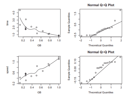
Recall that an objective way to compare different models is to compare their log likelihoods. Recall also that the appropriate likelihood is always for the untransformed $Y$, which means you need to figure out how the classical model for the transformed data $\left(f(Y)=\beta_0+\beta_1 X+\varepsilon\right)$ translates into a model $Y \mid X=x \sim p(y \mid x, \theta)$ for the original data. The likelihood you need is then the product of the $p\left(y_i \mid x_i, \theta\right)$ terms ( $n$ terms).
The Box-Cox method considers the family of transformed models
$$
Y^\lambda=\beta_0+\beta_1 X+\varepsilon, \text { for } \lambda \neq 0,
$$
with $\lambda=0$ given by the logarithmic model
$$
\ln (Y)=\beta_0+\beta_1 X+\varepsilon
$$
Special cases of interest are $\lambda=1$ (implying no transformation), $\lambda=0$ (log transform), $\lambda=-1$ (inverse transform), and $\lambda=0.5$ (square root transform).
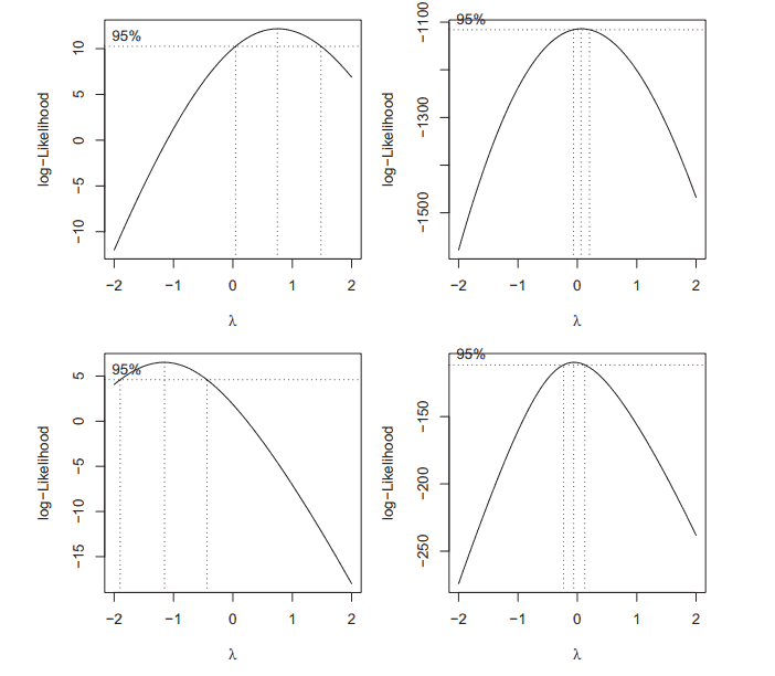
Each $\lambda$ induces a model for the original data of the form $Y \mid X=x \sim p_\lambda(y \mid x, \theta)$, and all of these $p_\lambda(y \mid x, \theta)$ distributions are non-normal except in the untransformed case where $\lambda=1$. For example, as shown above, the case $\lambda=0$ implies $p_0(y \mid x, \theta)$ is a lognormal distribution. The maximized log likelihoods for the original $Y$ data, which involve these (non-normal) distributions $p_\lambda(y \mid x, \theta)$, one for each possible $\lambda$, can then be compared to select “good” values of $\lambda$. You can use the “boxcox” function on a fitted Im object in $\mathrm{R}$ to estimate the “best” $\lambda$, but you first need to install the MASS library.
统计代写|线性回归分析代写linear regression analysis代考|Transforming Both $Y$ and $X$
It should be clear from the examples above that you can transform either $Y$ alone or $X$ alone. But you might have had an idea in your head that if you transform $Y$, then you should also transform $X$. In some cases, this is reasonable. After all, if $Y$ and $X$ have a relationship that is close to linear to begin with, then transforming one without the other will automatically introduce severe nonlinear curvature, badly violating the linearity assumption.
For example, consider total crimes $(Y)$ in a U.S. state as it relates to the population covered $(X)$, as reported by the FBI. The following code shows four scatterplots: $(X, Y),(X, \ln (Y))$, $(\ln (X), Y)$, and $(\ln (X), \ln (Y))$. It is clear, in this example, that if you transform one variable, then you must also transform the other.
Cr=read.table (“https://raw.githubusercontent. com/andrea2719/
URA-DataSets/master/Crimes_2012.txt”)
attach(Cr); par(mfrow=C $(2,2))$
plot (Tot_Crimes $~$ Pop_Cov)
lcrimes = log(Tot_Crimes); lpop = log(Pop_Cov)
plot (Tot_Crimes lpop); plot(lcrimes Pop_Cov); plot(lcrimes lpop)
Cr=read.table (“https://raw.githubusercontent. com/andrea2719/
URA-Datasets/master/crimes_2012.txt”)
$\operatorname{attach}(\mathrm{Cr}) ;$ par $(\operatorname{mfrow}=\mathrm{c}(2,2))$
plot (Tot_Crimes Pop_Cov)
lcrimes $=\log ($ Tot_Crimes $) ; \operatorname{lpop}=\log ($ Pop_Cov $)$
plot (Tot_Crimes lpop); plot (lcrimes Pop_Cov); plot (lcrimes lpop)
But it is not always needed to transform $X$ when you transform $Y$. In the computer example there was no need to transform the $X$ variable, RAM, even though we transformed $Y$, time, to $1 / Y$.
Among all of the possible combinations of $X$ – and $Y$-transforms, you can compare likelihood-based statistics to see, objectively, which model is best supported by the data. You can also evaluate the models according to how badly violated are assumptions, as discussed in Chapter 4, because higher log likelihood does not necessarily validate the assumptions of the model. Rather, the highest log likelihood among a collection of models that you are considering simply identifies the model that fits the data best among those you have considered. There may be other, better models that you have not considered. Further, even if the correct model is in your set of models, it will not necessarily have the best log likelihood because of randomness: Every random sample gives you a different $\log$ likelihood.
If you are considering transformations of the form $(f(X), g(Y))$, simply create the two new variables $U=f(X)$ and $W=g(Y)$, and evaluate the assumptions in terms of the transformed $(U, W)$ data as indicated in Chapter 4. If all looks reasonable, then the classical regression model
$$
W=\beta_0+\beta_1 U+\varepsilon
$$
is a reasonable model.

线性回归代写
统计代写|线性回归分析代写linear regression analysis代考|The Box-Cox Transformation
回想一下,比较不同模型的客观方法是比较它们的对数似然。还记得,适当的可能性总是针对未转换的$Y$,这意味着您需要弄清楚如何将转换后数据的经典模型$\left(f(Y)=\beta_0+\beta_1 X+\varepsilon\right)$转换为原始数据的模型$Y \mid X=x \sim p(y \mid x, \theta)$。然后,您需要的可能性是$p\left(y_i \mid x_i, \theta\right)$项的乘积($n$项)。
Box-Cox方法考虑转换后的模型族
$$
Y^\lambda=\beta_0+\beta_1 X+\varepsilon, \text { for } \lambda \neq 0,
$$
用$\lambda=0$给出的对数模型
$$
\ln (Y)=\beta_0+\beta_1 X+\varepsilon
$$
我们感兴趣的特殊情况有$\lambda=1$(意味着没有变换)、$\lambda=0$(对数变换)、$\lambda=-1$(逆变换)和$\lambda=0.5$(平方根变换)。
每个$\lambda$都为表单$Y \mid X=x \sim p_\lambda(y \mid x, \theta)$的原始数据引入了一个模型,除了$\lambda=1$未转换的情况外,所有这些$p_\lambda(y \mid x, \theta)$分布都是非正态分布。例如,如上所示,情况$\lambda=0$意味着$p_0(y \mid x, \theta)$是对数正态分布。原始$Y$数据的最大日志似然,包括这些(非正态)分布$p_\lambda(y \mid x, \theta)$,每个可能的$\lambda$一个,然后可以与$\lambda$的选择“好”值进行比较。您可以在$\mathrm{R}$中对一个拟合的Im对象使用“boxcox”函数来估计“最佳”$\lambda$,但是您首先需要安装MASS库。
统计代写|线性回归分析代写linear regression analysis代考|Transforming Both $Y$ and $X$
从上面的示例可以清楚地看出,您可以单独转换$Y$或单独转换$X$。但是你可能在脑子里有一个想法如果你变换$Y$,那么你也应该变换$X$。在某些情况下,这是合理的。毕竟,如果$Y$和$X$的关系一开始就接近线性,那么只变换其中一个会自动引入严重的非线性曲率,严重违反线性假设。
例如,考虑美国一个州的总犯罪$(Y)$,因为它与所覆盖的人口$(X)$有关,这是FBI报告的。下面的代码显示了四个散点图:$(X, Y),(X, \ln (Y))$、$(\ln (X), Y)$和$(\ln (X), \ln (Y))$。很明显,在这个例子中,如果你变换一个变量,那么你也必须变换另一个变量。
Cr=read。表(“https://raw.githubusercontent。com/andrea2719/
URA-DataSets/master/Crimes_2012.txt”)
附件(Cr);par(mfrow=C $(2,2))$
剧情(Tot_Crimes $~$ Pop_Cov)
lcrimes = log(Tot_Crimes);lpop = log(Pop_Cov)
plot (Tot_Crimes);情节(lcrimes Pop_Cov);情节(犯罪)
Cr=read。表(“https://raw.githubusercontent。com/andrea2719/
URA-Datasets/master/crimes_2012.txt”)
$\operatorname{attach}(\mathrm{Cr}) ;$ par $(\operatorname{mfrow}=\mathrm{c}(2,2))$
剧情(Tot_Crimes Pop_Cov)
lcrimes $=\log ($ Tot_Crimes $) ; \operatorname{lpop}=\log ($ Pop_Cov $)$
plot (Tot_Crimes);情节(lcrimes Pop_Cov);情节(犯罪)
但是在转换$Y$时并不总是需要转换$X$。在计算机示例中,不需要转换$X$变量RAM,尽管我们将$Y$时间转换为$1 / Y$。
在$X$ -和$Y$ -转换的所有可能组合中,您可以比较基于似然的统计数据,客观地查看哪个模型最受数据支持。您也可以根据假设被违背的程度来评估模型,正如第4章所讨论的那样,因为更高的对数似然不一定能验证模型的假设。相反,在您正在考虑的模型集合中,最高的对数似然只是标识出您所考虑的模型中最适合数据的模型。也许还有其他更好的模型是你没有考虑到的。此外,即使正确的模型在您的模型集中,由于随机性,它也不一定具有最佳对数似然:每个随机样本都会给您一个不同的$\log$似然。
如果您正在考虑对表单$(f(X), g(Y))$进行转换,只需创建两个新变量$U=f(X)$和$W=g(Y)$,并根据转换后的$(U, W)$数据评估假设,如第4章所示。如果一切看起来合理,那么经典回归模型
$$
W=\beta_0+\beta_1 U+\varepsilon
$$
是一个合理的模型。

统计代写请认准statistics-lab™. statistics-lab™为您的留学生涯保驾护航。
随机过程代考
在概率论概念中,随机过程是随机变量的集合。 若一随机系统的样本点是随机函数,则称此函数为样本函数,这一随机系统全部样本函数的集合是一个随机过程。 实际应用中,样本函数的一般定义在时间域或者空间域。 随机过程的实例如股票和汇率的波动、语音信号、视频信号、体温的变化,随机运动如布朗运动、随机徘徊等等。
贝叶斯方法代考
贝叶斯统计概念及数据分析表示使用概率陈述回答有关未知参数的研究问题以及统计范式。后验分布包括关于参数的先验分布,和基于观测数据提供关于参数的信息似然模型。根据选择的先验分布和似然模型,后验分布可以解析或近似,例如,马尔科夫链蒙特卡罗 (MCMC) 方法之一。贝叶斯统计概念及数据分析使用后验分布来形成模型参数的各种摘要,包括点估计,如后验平均值、中位数、百分位数和称为可信区间的区间估计。此外,所有关于模型参数的统计检验都可以表示为基于估计后验分布的概率报表。
广义线性模型代考
广义线性模型(GLM)归属统计学领域,是一种应用灵活的线性回归模型。该模型允许因变量的偏差分布有除了正态分布之外的其它分布。
statistics-lab作为专业的留学生服务机构,多年来已为美国、英国、加拿大、澳洲等留学热门地的学生提供专业的学术服务,包括但不限于Essay代写,Assignment代写,Dissertation代写,Report代写,小组作业代写,Proposal代写,Paper代写,Presentation代写,计算机作业代写,论文修改和润色,网课代做,exam代考等等。写作范围涵盖高中,本科,研究生等海外留学全阶段,辐射金融,经济学,会计学,审计学,管理学等全球99%专业科目。写作团队既有专业英语母语作者,也有海外名校硕博留学生,每位写作老师都拥有过硬的语言能力,专业的学科背景和学术写作经验。我们承诺100%原创,100%专业,100%准时,100%满意。
机器学习代写
随着AI的大潮到来,Machine Learning逐渐成为一个新的学习热点。同时与传统CS相比,Machine Learning在其他领域也有着广泛的应用,因此这门学科成为不仅折磨CS专业同学的“小恶魔”,也是折磨生物、化学、统计等其他学科留学生的“大魔王”。学习Machine learning的一大绊脚石在于使用语言众多,跨学科范围广,所以学习起来尤其困难。但是不管你在学习Machine Learning时遇到任何难题,StudyGate专业导师团队都能为你轻松解决。
多元统计分析代考
基础数据: $N$ 个样本, $P$ 个变量数的单样本,组成的横列的数据表
变量定性: 分类和顺序;变量定量:数值
数学公式的角度分为: 因变量与自变量
时间序列分析代写
随机过程,是依赖于参数的一组随机变量的全体,参数通常是时间。 随机变量是随机现象的数量表现,其时间序列是一组按照时间发生先后顺序进行排列的数据点序列。通常一组时间序列的时间间隔为一恒定值(如1秒,5分钟,12小时,7天,1年),因此时间序列可以作为离散时间数据进行分析处理。研究时间序列数据的意义在于现实中,往往需要研究某个事物其随时间发展变化的规律。这就需要通过研究该事物过去发展的历史记录,以得到其自身发展的规律。
回归分析代写
多元回归分析渐进(Multiple Regression Analysis Asymptotics)属于计量经济学领域,主要是一种数学上的统计分析方法,可以分析复杂情况下各影响因素的数学关系,在自然科学、社会和经济学等多个领域内应用广泛。
MATLAB代写
MATLAB 是一种用于技术计算的高性能语言。它将计算、可视化和编程集成在一个易于使用的环境中,其中问题和解决方案以熟悉的数学符号表示。典型用途包括:数学和计算算法开发建模、仿真和原型制作数据分析、探索和可视化科学和工程图形应用程序开发,包括图形用户界面构建MATLAB 是一个交互式系统,其基本数据元素是一个不需要维度的数组。这使您可以解决许多技术计算问题,尤其是那些具有矩阵和向量公式的问题,而只需用 C 或 Fortran 等标量非交互式语言编写程序所需的时间的一小部分。MATLAB 名称代表矩阵实验室。MATLAB 最初的编写目的是提供对由 LINPACK 和 EISPACK 项目开发的矩阵软件的轻松访问,这两个项目共同代表了矩阵计算软件的最新技术。MATLAB 经过多年的发展,得到了许多用户的投入。在大学环境中,它是数学、工程和科学入门和高级课程的标准教学工具。在工业领域,MATLAB 是高效研究、开发和分析的首选工具。MATLAB 具有一系列称为工具箱的特定于应用程序的解决方案。对于大多数 MATLAB 用户来说非常重要,工具箱允许您学习和应用专业技术。工具箱是 MATLAB 函数(M 文件)的综合集合,可扩展 MATLAB 环境以解决特定类别的问题。可用工具箱的领域包括信号处理、控制系统、神经网络、模糊逻辑、小波、仿真等。