如果你也在 怎样代写机器学习 machine learning这个学科遇到相关的难题,请随时右上角联系我们的24/7代写客服。
机器学习是一个致力于理解和建立 “学习 “方法的研究领域,也就是说,利用数据来提高某些任务的性能的方法。机器学习算法基于样本数据(称为训练数据)建立模型,以便在没有明确编程的情况下做出预测或决定。机器学习算法被广泛用于各种应用,如医学、电子邮件过滤、语音识别和计算机视觉,在这些应用中,开发传统算法来执行所需任务是困难的或不可行的。
statistics-lab™ 为您的留学生涯保驾护航 在代写机器学习 machine learning方面已经树立了自己的口碑, 保证靠谱, 高质且原创的统计Statistics代写服务。我们的专家在代写机器学习 machine learning代写方面经验极为丰富,各种代写机器学习 machine learning相关的作业也就用不着说。
我们提供的机器学习 machine learning及其相关学科的代写,服务范围广, 其中包括但不限于:
- Statistical Inference 统计推断
- Statistical Computing 统计计算
- Advanced Probability Theory 高等概率论
- Advanced Mathematical Statistics 高等数理统计学
- (Generalized) Linear Models 广义线性模型
- Statistical Machine Learning 统计机器学习
- Longitudinal Data Analysis 纵向数据分析
- Foundations of Data Science 数据科学基础
计算机代写|机器学习代写machine learning代考|The K-medoids algorithm
There is a variant of K-means called $\mathbf{K}$-medoids algorithm, in which we estimate each cluster center $\boldsymbol{\mu}_k$ by choosing the data example $\boldsymbol{x}_n \in \mathcal{X}$ whose average dissimilarity to all other points in that cluster is minimal; such a point is known as a medoid. By contrast, in K-means, we take averages over points $\boldsymbol{x}_n \in \mathbb{R}^D$ assigned to the cluster to compute the center. K-medoids can be more robust to outliers (although that issue can also be tackled by using mixtures of Student distributions, instead of mixtures of Gaussians). More importantly, K-medoids can be applied to data that does not live in $\mathbb{R}^D$, where averaging may not be well defined. In K-medoids, the input to the algorithm is $N \times N$ pairwise distance matrix, $D\left(n, n^{\prime}\right)$, not an $N \times D$ feature matrix.
The classic algorithm for solving the K-medoids is the partitioning around medoids or PAM method [KR87]. In this approach, at each iteration, we loop over all $K$ medoids. For each medoid $m$, we consider each non-medoid point $o$, swap $m$ and $o$, and recompute the cost (sum of all the distances of points to their medoid). If the cost has decreased, we keep this swap. The running time of this algorithm is $O\left(N^2 K T\right)$, where $T$ is the number of iterations.
There is also a simpler and faster method, known as the Voronoi iteration method due to [PJ09]. In this approach, at each iteration, we have two steps, similar to K-means. First, for each cluster $k$, look at all the points currently assigned to that cluster, $S_k=\left{n: z_n=k\right}$, and then set $m_k$ to be the index of the medoid of that set. (To find the medoid requires examining all $\left|S_k\right|$ candidate points, and choosing the one that has the smallest sum of distances to all the other points in $S_k$.) Second, for each point $n$, assign it to its closest medoid, $z_n=\operatorname{argmin}_k D(n, k)$. The pseudo-code is given in Algorithm 12.
计算机代写|机器学习代写machine learning代考|Minimizing the distortion
Based on our experience with supervised learning, a natural choice for picking $K$ is to pick the value that minimizes the reconstruction error on a validation set, defined as follows:
$$
\operatorname{err}\left(\mathcal{D}{\text {valid }}, K\right)=\frac{1}{\left|\mathcal{D}{\text {valid }}\right|} \sum_{n \in \mathcal{D}_{\text {valia }}}\left|\boldsymbol{x}_n-\hat{\boldsymbol{x}}_n\right|_2^2
$$
where $\hat{\boldsymbol{x}}_n=$ decode $\left(\right.$ encode $\left.\left(\boldsymbol{x}_n\right)\right)$ is the reconstruction of $\boldsymbol{x}_n$.
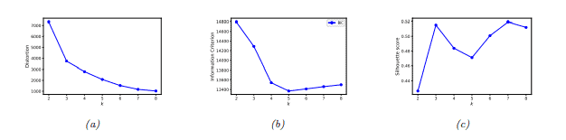
Unfortunately, this technique will not work. Indeed, as we see in Figure 21.11a, the distortion monotonically decreases with $K$. To see why, note that the K-means model is a degenerate density model which consists of $K$ “spikes” at the $\boldsymbol{\mu}_k$ centers. As we increase $K$, we “cover” more of the input space. Hence any given input point is more likely to find a close prototype to accurately represent it as $K$ increases, thus decreasing reconstruction error. Thus unlike with supervised learning, we cannot use reconstruction error on a validation set as a way to select the best unsupervised model. (This comment also applies to picking the dimensionality for PCA, see Section 20.1.4.)
A method that does work is to use a proper probabilistic model, such as a GMM, as we describe in Section 21.4.1. We can then use the log marginal likelihood (LML) of the data to perform model selection.
We can approximate the LML using the BIC score as we discussed in Section 5.2.5.1. From Equation (5.59), we have
$$
\operatorname{BIC}(K)=\log p\left(\mathcal{D} \mid \hat{\boldsymbol{\theta}}_k\right)-\frac{D_K}{2} \log (N)
$$
where $D_K$ is the number of parameters in a model with $K$ clusters, and $\hat{\boldsymbol{\theta}}_K$ is the MLE. We see from Figure 21.11b that this exhibits the typical U-shaped curve, where the penalty decreases and then increases.
The reason this works is that each cluster is associated with a Gaussian distribution that fills a volume of the input space, rather than being a degenerate spike. Once we have enough clusters to cover the true modes of the distribution, the Bayesian Occam’s razor (Section 5.2.3) kicks in, and starts penalizing the model for being unncessarily complex.
See Section 21.4.1.3 for more discussion of Bayesian model selection for mixture models.
机器学习代考
计算机代写|机器学习代写machine learning代考|The K-medoids algorithm
K-means 有一个变体叫做钾-medoids 算法,我们在其中估计每个聚类中心米k通过选择数据示例Xn∈X与该集群中所有其他点的平均差异最小;这样的点被称为中心点。相比之下,在 K-means 中,我们对点取平均值Xn∈R丁分配给集群计算中心。K-medoids 对离群值更稳健(尽管这个问题也可以通过使用学生分布的混合来解决,而不是高斯分布的混合)。更重要的是,K-medoids 可以应用于不存在于R丁,其中平均可能没有明确定义。在 K-medoids 中,算法的输入是否×否成对距离矩阵,丁(n,n′), 不是否×丁特征矩阵。
求解 K-medoids 的经典算法是 partitioning around medoids 或 PAM 方法 [KR87]。在这种方法中,在每次迭代中,我们遍历所有钾中心点。对于每个中心点米,我们考虑每个非中心点欧, 交换米和欧,并重新计算成本(点到其中心点的所有距离的总和)。如果成本降低,我们将保留此掉期。该算法的运行时间为欧(否2钾吨), 在哪里吨是迭代次数。
还有一种更简单、更快的方法,由于 [PJ09] 而被称为 Voronoi 迭代法。在这种方法中,在每次迭代中,我们有两个步骤,类似于 K-means。首先,对于每个集群k,查看当前分配给该集群的所有点,S_k=\left{n: z_n=k\right}S_k=\left{n: z_n=k\right}, 然后设置米k成为该集合的中心点的索引。(要找到中心点需要检查所有|小号k|候选点,并选择与所有其他点的距离之和最小的点小号k.) 其次,对于每个点n,将其分配给最接近的中心点,和n=精氨酸k丁(n,k). 伪代码在算法 12 中给出。
计算机代写|机器学习代写machine learning代考|Minimizing the distortion
根据我们在监督学习方面的经验,采摘的自然选择 $K$ 是选择最小化验证集上的重构误差的值,定义如下:
$$
\operatorname{err}(\mathcal{D} \text { valid }, K)=\frac{1}{\mid \mathcal{D} \text { valid } \mid} \sum_{n \in \mathcal{D}_{\text {valia }}}\left|\boldsymbol{x}_n-\hat{\boldsymbol{x}}_n\right|_2^2
$$
在哪里 $\hat{\boldsymbol{x}}_n=$ 解码 (编码 $\left.\left(\boldsymbol{x}_n\right)\right)$ 是重建 $\boldsymbol{x}_n$.
不幸的是,这种技术行不通。实际上,正如我们在图 21.11a 中看到的,失真随着 $K$. 要了解原因,请注意 $\mathrm{K}-$ means 模型是一个退化密度模型,它由以下部分组成 $K^{\prime \prime}$ 尖峰”在 $\boldsymbol{\mu}_k$ 中心。随着我们增加 $K$ ,我们 “覆盖”了更多 的输入空间。因此,任何给定的输入点更有可能找到一个接近的原型来准确地将其表示为 $K$ 增加,从而减少重建 误差。因此,与监督学习不同,我们不能使用验证集上的重构误差作为选择最佳无监督模型的方法。(此评论也 适用于为 PCA 选择维度,请参阅第 20.1.4 节。)
一种有效的方法是使用适当的概率模型,例如 GMM,如我们在第 $21.4 .1$ 节中所述。然后,我们可以使用数据 的对数边际似然 $(L M L)$ 来执行模型选择。
正如我们在第 5.2.5.1 节中讨论的那样,我们可以使用 BIC 分数来近似 LML。从等式 (5.59),我们有
$$
\operatorname{BIC}(K)=\log p\left(\mathcal{D} \mid \hat{\boldsymbol{\theta}}_k\right)-\frac{D_K}{2} \log (N)
$$
在哪里 $D_K$ 是模型中的参数数量 $K$ 集群,和 $\hat{\boldsymbol{\theta}}_K$ 是 $\mathrm{MLE}$ 。我们从图 21.11b 中看到,这呈现出典型的 U 形曲线, 其中惩罚先减小后增加。
这样做的原因是每个集群都与填充输入空间体积的高斯分布相关联,而不是退化尖峰。一旦我们有足够的集群来 覆盖分布的真实模式,贝叶斯奥卡姆挮刀(第 5.2.3 节) 就会启动,并开始征罚不必要的复杂模型。
有关混合模型的贝叶斯模型选择的更多讨论,请参见第 21.4.1.3 节。

统计代写请认准statistics-lab™. statistics-lab™为您的留学生涯保驾护航。
金融工程代写
金融工程是使用数学技术来解决金融问题。金融工程使用计算机科学、统计学、经济学和应用数学领域的工具和知识来解决当前的金融问题,以及设计新的和创新的金融产品。
非参数统计代写
非参数统计指的是一种统计方法,其中不假设数据来自于由少数参数决定的规定模型;这种模型的例子包括正态分布模型和线性回归模型。
广义线性模型代考
广义线性模型(GLM)归属统计学领域,是一种应用灵活的线性回归模型。该模型允许因变量的偏差分布有除了正态分布之外的其它分布。
术语 广义线性模型(GLM)通常是指给定连续和/或分类预测因素的连续响应变量的常规线性回归模型。它包括多元线性回归,以及方差分析和方差分析(仅含固定效应)。
有限元方法代写
有限元方法(FEM)是一种流行的方法,用于数值解决工程和数学建模中出现的微分方程。典型的问题领域包括结构分析、传热、流体流动、质量运输和电磁势等传统领域。
有限元是一种通用的数值方法,用于解决两个或三个空间变量的偏微分方程(即一些边界值问题)。为了解决一个问题,有限元将一个大系统细分为更小、更简单的部分,称为有限元。这是通过在空间维度上的特定空间离散化来实现的,它是通过构建对象的网格来实现的:用于求解的数值域,它有有限数量的点。边界值问题的有限元方法表述最终导致一个代数方程组。该方法在域上对未知函数进行逼近。[1] 然后将模拟这些有限元的简单方程组合成一个更大的方程系统,以模拟整个问题。然后,有限元通过变化微积分使相关的误差函数最小化来逼近一个解决方案。
tatistics-lab作为专业的留学生服务机构,多年来已为美国、英国、加拿大、澳洲等留学热门地的学生提供专业的学术服务,包括但不限于Essay代写,Assignment代写,Dissertation代写,Report代写,小组作业代写,Proposal代写,Paper代写,Presentation代写,计算机作业代写,论文修改和润色,网课代做,exam代考等等。写作范围涵盖高中,本科,研究生等海外留学全阶段,辐射金融,经济学,会计学,审计学,管理学等全球99%专业科目。写作团队既有专业英语母语作者,也有海外名校硕博留学生,每位写作老师都拥有过硬的语言能力,专业的学科背景和学术写作经验。我们承诺100%原创,100%专业,100%准时,100%满意。
随机分析代写
随机微积分是数学的一个分支,对随机过程进行操作。它允许为随机过程的积分定义一个关于随机过程的一致的积分理论。这个领域是由日本数学家伊藤清在第二次世界大战期间创建并开始的。
时间序列分析代写
随机过程,是依赖于参数的一组随机变量的全体,参数通常是时间。 随机变量是随机现象的数量表现,其时间序列是一组按照时间发生先后顺序进行排列的数据点序列。通常一组时间序列的时间间隔为一恒定值(如1秒,5分钟,12小时,7天,1年),因此时间序列可以作为离散时间数据进行分析处理。研究时间序列数据的意义在于现实中,往往需要研究某个事物其随时间发展变化的规律。这就需要通过研究该事物过去发展的历史记录,以得到其自身发展的规律。
回归分析代写
多元回归分析渐进(Multiple Regression Analysis Asymptotics)属于计量经济学领域,主要是一种数学上的统计分析方法,可以分析复杂情况下各影响因素的数学关系,在自然科学、社会和经济学等多个领域内应用广泛。
MATLAB代写
MATLAB 是一种用于技术计算的高性能语言。它将计算、可视化和编程集成在一个易于使用的环境中,其中问题和解决方案以熟悉的数学符号表示。典型用途包括:数学和计算算法开发建模、仿真和原型制作数据分析、探索和可视化科学和工程图形应用程序开发,包括图形用户界面构建MATLAB 是一个交互式系统,其基本数据元素是一个不需要维度的数组。这使您可以解决许多技术计算问题,尤其是那些具有矩阵和向量公式的问题,而只需用 C 或 Fortran 等标量非交互式语言编写程序所需的时间的一小部分。MATLAB 名称代表矩阵实验室。MATLAB 最初的编写目的是提供对由 LINPACK 和 EISPACK 项目开发的矩阵软件的轻松访问,这两个项目共同代表了矩阵计算软件的最新技术。MATLAB 经过多年的发展,得到了许多用户的投入。在大学环境中,它是数学、工程和科学入门和高级课程的标准教学工具。在工业领域,MATLAB 是高效研究、开发和分析的首选工具。MATLAB 具有一系列称为工具箱的特定于应用程序的解决方案。对于大多数 MATLAB 用户来说非常重要,工具箱允许您学习和应用专业技术。工具箱是 MATLAB 函数(M 文件)的综合集合,可扩展 MATLAB 环境以解决特定类别的问题。可用工具箱的领域包括信号处理、控制系统、神经网络、模糊逻辑、小波、仿真等。