如果你也在 怎样代写微观经济学Microeconomics这个学科遇到相关的难题,请随时右上角联系我们的24/7代写客服。
微观经济学是研究稀缺性及其对资源的使用、商品和服务的生产、生产和福利的长期增长的影响,以及对社会至关重要的其他大量复杂问题的研究。
statistics-lab™ 为您的留学生涯保驾护航 在代写微观经济学Microeconomics方面已经树立了自己的口碑, 保证靠谱, 高质且原创的统计Statistics代写服务。我们的专家在代写微观经济学Microeconomics代写方面经验极为丰富,各种代写微观经济学Microeconomics相关的作业也就用不着说。
我们提供的微观经济学Microeconomics及其相关学科的代写,服务范围广, 其中包括但不限于:
- Statistical Inference 统计推断
- Statistical Computing 统计计算
- Advanced Probability Theory 高等概率论
- Advanced Mathematical Statistics 高等数理统计学
- (Generalized) Linear Models 广义线性模型
- Statistical Machine Learning 统计机器学习
- Longitudinal Data Analysis 纵向数据分析
- Foundations of Data Science 数据科学基础
经济代写|微观经济学代写Microeconomics代考|Necessary Conditions
We know from optimization problems without constraints, $\max _x f(x)$, that firstorder conditions $f^{\prime}(x)=0$ are merely sufficient, not necessary for a maximum or minimum of a function. In addition, the objective function must be strictly concave (maximum) or convex (minimum). This can be checked under certain conditions using the second derivatives of the objective function, and we get $f^{\prime \prime}(x) \leq 0$ for a maximum and $f^{\prime \prime}(x) \geq 0$ for a minimum. For optimization problems with multiple endogenous variables and with constraints, this test has to be generalized. Whether there is a maximum or a minimum is determined by the signs of the principal minors of the so-called bordered Hessian matrix.
The bordered Hessian matrix is a particular arrangement of the second derivatives of the Lagrangian function. In order to have a lean notation, we will use the following abbreviations. The first derivatives of the functions $\mathcal{L}, f$ and $g$ with respect to $x_i, i=1, \ldots, n$ and $\lambda$ are denoted by $\mathcal{L}{x_i}, \mathcal{L}\lambda, f_{x_i}, f_\lambda$, and $g_{x_i}, g_\lambda$, respectively. Analogously, the second derivatives are denoted as $x_j, j=1, \ldots n$ $\mathcal{L}{x_i x_j}, \mathcal{L}{\lambda x_j}, f_{x_i x_j}, f_{\lambda x_j}$, and $g_{x_i x_j}, g_{\lambda x_j}, \lambda \mathcal{L}{x_i \lambda}, \mathcal{L}{\lambda \lambda}, f_{x_i \lambda}, f_{\lambda \lambda}, g_{x_i \lambda}, g_{\lambda \lambda}$. With this notation, the first-order conditions can also be written as follows:
$$
\begin{aligned}
\mathcal{L}{x_i} & =f{x_i}-\lambda \cdot g_{x_i}=0, \quad i=1, \ldots, n, \
\mathcal{L}\lambda & =g-c=0 . \end{aligned} $$ This system of equations yields $(n+1) \cdot(n+1)$ second-order conditions, which are systematically denoted as the bordered Hessian matrix: $$ H\left(x_1, \ldots, x_n, \lambda\right)=\left(\begin{array}{cccc} \mathcal{L}{\lambda \lambda} & \mathcal{L}{\lambda x_1} & \ldots & \mathcal{L}{\lambda x_n} \
\mathcal{L}{x_1 \lambda} & \mathcal{L}{x_1 x_1} & \ldots & \mathcal{L}{x_1 x_n} \ \ldots & \ldots & \ldots & \ldots \ \mathcal{L}{x_n \lambda} & \mathcal{L}{x_n x_1} & \ldots & \mathcal{L}{x_n x_n}
\end{array}\right)=\left(\begin{array}{cccc}
0 & g_{x_1} & \ldots & g_{x_n} \
g_{x_1} & f_{x_1 x_1}-\lambda g_{x_1 x_1} & \ldots & f_{x_n x_1}-\lambda g_{x_n x_1} \
\ldots & \ldots & \ldots & \ldots \
g_{x_n} & f_{x_n x_1}-\lambda g_{x_1 x_1} & \ldots & f_{x_n x_n}-\lambda g_{x_n x_n}
\end{array}\right)
$$
The bordered Hessian matrix is square and mirror symmetric with respect to its main axis, $\mathcal{L}{x_1 x_j}=\mathcal{L}{x_j x_1}, \mathcal{L}{x_i \lambda}=\mathcal{L}{\lambda x_i}$. It can be split into submatrices
$$
H_1=\mathcal{L}{\lambda \lambda}, H_2=\left(\begin{array}{cc} \mathcal{L}{\lambda \lambda} & \mathcal{L}{\lambda x_1} \ \mathcal{L}{x_1 \lambda} & \mathcal{L}{x_1 x_1} \end{array}\right), \ldots, $$ where the last submatrix $H{n+1}$ is identical to matrix $H$.
经济代写|微观经济学代写Microeconomics代考|Optimization Under Constraints
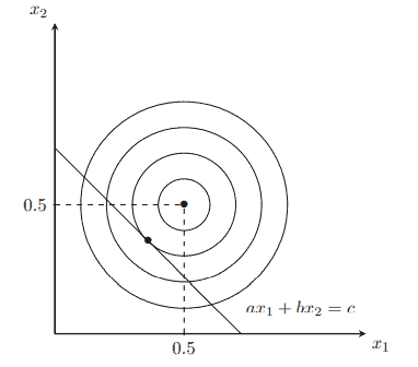
For a number of optimization problems one does not search for the unconstrained optimum of a function $f\left(x_1, \ldots, x_n\right)$ (the objective function), but for the optimum relative to certain constraints. As an example, consider a utility function with a point of satiation (the global maximum), as shown in Fig. 7.3d. Formally, such a function can, e.g., be described by the function $u\left(x_1, x_2\right)=x_1-\left(x_1\right)^2+x_2-\left(x_2\right)^2$, whose indifference curves are shown in Fig. 17.2.
The unconstrained maximum of this function is at $x_1=x_2=0.5$. If the set of admissible solutions is restricted to lie on the function $a x_1+b x_2=c$ (i.e., a linear constraint is introduced, which must lie “below” the global maximum), the global maximum is no longer attainable. Instead, the relative maximum now lies on the straight line drawn in Fig. 17.3.
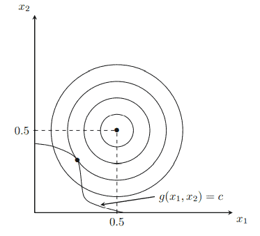
Analogous considerations hold if the choice set is not constrained by a linear restriction, but by a general restriction of the form $g\left(x_1, \ldots, x_2\right)=c$. This is illustrated in Fig. 17.4.
We assume in the following that we want to solve an optimization problem with $n$ variables $x_1, \ldots, x_n$. In order to determine the constrained optimum, we need to develop a method that ensures that we only search for solutions within the admissible subset defined by the constraint. Such a method is the Lagrange method.
微观经济学代考
经济代写|微观经济学代写Microeconomics代考|Necessary Conditions
我们从没有约束的优化问题中知道, $\max x f(x)$ ,一阶条件 $f^{\prime}(x)=0$ 对于功能的最大或最小值而言,它 们仅仅是足够的,而不是必需的。此外,目标函数必须是严格凹的(最大)或凸的(最小)。这可以在特 定条件下使用目标函数的二阶导数进行检查,我们得到 $f^{\prime \prime}(x) \leq 0$ 对于最大和 $f^{\prime \prime}(x) \geq 0$ 至少。对于具 有多个内生变量和约束的优化问题,必须推广此测试。是否存在最大值或最小值由所谓的有边 Hessian 矩 阵的主辅矩阵的符号决定。 带边界的 Hessian 矩阵是拉格朗日函数的二阶导数的特殊排列。为了有一个精简的符号,我们将使用以下 缩写。函数的一阶导数 $\mathcal{L}, f$ 和 $g$ 关于 $x_i, i=1, \ldots, n$ 和 $\lambda$ 表示为 $\mathcal{L} x_i, \mathcal{L} \lambda, f{x_i}, f_\lambda$ ,和 $g_{x_i}, g_\lambda$ ,分别。 类似地,二阶导数表示为 $x_j, j=1, \ldots n \mathcal{L} x_i x_j, \mathcal{L} \lambda x_j, f_{x_i x_j}, f_{\lambda x_j}$ ,和 $g_{x_i x_j}, g_{\lambda x_j}, \lambda \mathcal{L} x_i \lambda, \mathcal{L} \lambda \lambda, f_{x_i \lambda}, f_{\lambda \lambda}, g_{x_i \lambda}, g_{\lambda \lambda}$. 使用这种表示法,一阶条件也可以写成如下:
$$
\mathcal{L} x_i=f x_i-\lambda \cdot g_{x_i}=0, \quad i=1, \ldots, n, \mathcal{L} \lambda \quad=g-c=0 .
$$
这个方程组产生 $(n+1) \cdot(n+1)$ 二阶条件,系统地表示为带边界的 Hessian 矩阵:
$$
H\left(x_1, \ldots, x_n, \lambda\right)=\left(\begin{array}{llllllllll}
\mathcal{L} \lambda \lambda & \mathcal{L} \lambda x_1 & \ldots & \mathcal{L} \lambda x_n \mathcal{L} x_1 \lambda & \mathcal{L} x_1 x_1 & \ldots & \mathcal{L} x_1 x_n & \ldots & \ldots & \ldots
\end{array}\right.
$$
有边界的 Hessian 矩阵是方形的,并且相对于它的主轴是镜像对称的,
$\mathcal{L} x_1 x_j=\mathcal{L} x_j x_1, \mathcal{L} x_i \lambda=\mathcal{L} \lambda x_i$. 它可以拆分成子矩阵
$$
H_1=\mathcal{L} \lambda \lambda, H_2=\left(\begin{array}{lll}
\mathcal{L} \lambda \lambda & \mathcal{L} \lambda x_1 & \mathcal{L} x_1 \lambda \quad \mathcal{L} x_1 x_1
\end{array}\right), \ldots,
$$
最后一个子矩阵在哪里 $H n+1$ 与矩阵相同 $H$.
经济代写|微观经济学代写Microeconomics代考|Optimization Under Constraints
对于许多优化问题,人们不会搜索函数的无约束最优值 $f\left(x_1, \ldots, x_n\right)$ (目标函数),但相对于某些约束 的最优。例如,考虑一个具有饱和点(全局最大值) 的效用函数,如图 7.3d 所示。形式上,这样的功能 可以,例如,由功能描述 $u\left(x_1, x_2\right)=x_1-\left(x_1\right)^2+x_2-\left(x_2\right)^2$ ,其无差异曲线如图 $17.2$ 所示。
此函数的无约束最大值位于 $x_1=x_2=0.5$. 如果可接受的解决方案集被限制在函数上 $a x_1+b x_2=c$ (即,引入了一个线性约束,它必须位于“低于”全局最大值),全局最大值不再是可达到的。相反,相对 最大值现在位于图 $17.3$ 中绘制的直线上。
如果选择集不受线性限制,而是受形式的一般限制,则类似的考虑成立 $g\left(x_1, \ldots, x_2\right)=c$. 如图 $17.4$ 所 示。
我们假设在下面我们想要解决一个优化问题 $n$ 变量 $x_1, \ldots, x_n$. 为了确定约束最优解,我们需要开发一种 方法来确保我们只在约束定义的可容许子集中搜索解。这种方法就是拉格朗日方法。

统计代写请认准statistics-lab™. statistics-lab™为您的留学生涯保驾护航。
金融工程代写
金融工程是使用数学技术来解决金融问题。金融工程使用计算机科学、统计学、经济学和应用数学领域的工具和知识来解决当前的金融问题,以及设计新的和创新的金融产品。
非参数统计代写
非参数统计指的是一种统计方法,其中不假设数据来自于由少数参数决定的规定模型;这种模型的例子包括正态分布模型和线性回归模型。
广义线性模型代考
广义线性模型(GLM)归属统计学领域,是一种应用灵活的线性回归模型。该模型允许因变量的偏差分布有除了正态分布之外的其它分布。
术语 广义线性模型(GLM)通常是指给定连续和/或分类预测因素的连续响应变量的常规线性回归模型。它包括多元线性回归,以及方差分析和方差分析(仅含固定效应)。
有限元方法代写
有限元方法(FEM)是一种流行的方法,用于数值解决工程和数学建模中出现的微分方程。典型的问题领域包括结构分析、传热、流体流动、质量运输和电磁势等传统领域。
有限元是一种通用的数值方法,用于解决两个或三个空间变量的偏微分方程(即一些边界值问题)。为了解决一个问题,有限元将一个大系统细分为更小、更简单的部分,称为有限元。这是通过在空间维度上的特定空间离散化来实现的,它是通过构建对象的网格来实现的:用于求解的数值域,它有有限数量的点。边界值问题的有限元方法表述最终导致一个代数方程组。该方法在域上对未知函数进行逼近。[1] 然后将模拟这些有限元的简单方程组合成一个更大的方程系统,以模拟整个问题。然后,有限元通过变化微积分使相关的误差函数最小化来逼近一个解决方案。
tatistics-lab作为专业的留学生服务机构,多年来已为美国、英国、加拿大、澳洲等留学热门地的学生提供专业的学术服务,包括但不限于Essay代写,Assignment代写,Dissertation代写,Report代写,小组作业代写,Proposal代写,Paper代写,Presentation代写,计算机作业代写,论文修改和润色,网课代做,exam代考等等。写作范围涵盖高中,本科,研究生等海外留学全阶段,辐射金融,经济学,会计学,审计学,管理学等全球99%专业科目。写作团队既有专业英语母语作者,也有海外名校硕博留学生,每位写作老师都拥有过硬的语言能力,专业的学科背景和学术写作经验。我们承诺100%原创,100%专业,100%准时,100%满意。
随机分析代写
随机微积分是数学的一个分支,对随机过程进行操作。它允许为随机过程的积分定义一个关于随机过程的一致的积分理论。这个领域是由日本数学家伊藤清在第二次世界大战期间创建并开始的。
时间序列分析代写
随机过程,是依赖于参数的一组随机变量的全体,参数通常是时间。 随机变量是随机现象的数量表现,其时间序列是一组按照时间发生先后顺序进行排列的数据点序列。通常一组时间序列的时间间隔为一恒定值(如1秒,5分钟,12小时,7天,1年),因此时间序列可以作为离散时间数据进行分析处理。研究时间序列数据的意义在于现实中,往往需要研究某个事物其随时间发展变化的规律。这就需要通过研究该事物过去发展的历史记录,以得到其自身发展的规律。
回归分析代写
多元回归分析渐进(Multiple Regression Analysis Asymptotics)属于计量经济学领域,主要是一种数学上的统计分析方法,可以分析复杂情况下各影响因素的数学关系,在自然科学、社会和经济学等多个领域内应用广泛。
MATLAB代写
MATLAB 是一种用于技术计算的高性能语言。它将计算、可视化和编程集成在一个易于使用的环境中,其中问题和解决方案以熟悉的数学符号表示。典型用途包括:数学和计算算法开发建模、仿真和原型制作数据分析、探索和可视化科学和工程图形应用程序开发,包括图形用户界面构建MATLAB 是一个交互式系统,其基本数据元素是一个不需要维度的数组。这使您可以解决许多技术计算问题,尤其是那些具有矩阵和向量公式的问题,而只需用 C 或 Fortran 等标量非交互式语言编写程序所需的时间的一小部分。MATLAB 名称代表矩阵实验室。MATLAB 最初的编写目的是提供对由 LINPACK 和 EISPACK 项目开发的矩阵软件的轻松访问,这两个项目共同代表了矩阵计算软件的最新技术。MATLAB 经过多年的发展,得到了许多用户的投入。在大学环境中,它是数学、工程和科学入门和高级课程的标准教学工具。在工业领域,MATLAB 是高效研究、开发和分析的首选工具。MATLAB 具有一系列称为工具箱的特定于应用程序的解决方案。对于大多数 MATLAB 用户来说非常重要,工具箱允许您学习和应用专业技术。工具箱是 MATLAB 函数(M 文件)的综合集合,可扩展 MATLAB 环境以解决特定类别的问题。可用工具箱的领域包括信号处理、控制系统、神经网络、模糊逻辑、小波、仿真等。