如果你也在 怎样代写期权定价理论Option Pricing Theory这个学科遇到相关的难题,请随时右上角联系我们的24/7代写客服。
期权定价理论通过分配一个价格,也就是溢价,根据计算出的合同在到期时完成货币(ITM)的概率来估计期权合同的价值。
statistics-lab™ 为您的留学生涯保驾护航 在代写期权定价理论Option Pricing Theory方面已经树立了自己的口碑, 保证靠谱, 高质且原创的统计Statistics代写服务。我们的专家在代写期权定价理论Option Pricing Theory代写方面经验极为丰富,各种代写期权定价理论Option Pricing Theory相关的作业也就用不着说。
我们提供的期权定价理论Option Pricing Theory及其相关学科的代写,服务范围广, 其中包括但不限于:
- Statistical Inference 统计推断
- Statistical Computing 统计计算
- Advanced Probability Theory 高等概率论
- Advanced Mathematical Statistics 高等数理统计学
- (Generalized) Linear Models 广义线性模型
- Statistical Machine Learning 统计机器学习
- Longitudinal Data Analysis 纵向数据分析
- Foundations of Data Science 数据科学基础
金融代写|期权定价理论代写Option Pricing Theory代考|SD Option Pricing by Pairwise Comparisons
Recall from Chap. 1 that the fundamental property of SSD is that for every agent the utility function must be increasing and concave, implying in turn that the marginal utility function is non-increasing. This fundamental property of decision-makers identified here as investors or traders in both the underlying and the option is the basis of the $\mathrm{SD}$ approach to option pricing. In market equilibrium models, this marginal utility is known as the pricing kernel and constitutes a basic element in defining the equilibrium prices of derivative assets.
We consider a market with an underlying asset with current price $S_t$ and a riskless asset with return per period equal to $R$. There is also a European call option with strike price $K$ expiring at some future time $T$. Time is initially assumed discrete $t=0,1, \ldots, T$, with intervals of length $\Delta t$, implying that $R=e^{r \Delta t}=1+r \Delta t+o(\Delta t)$, where $r$ denotes the interest rate in continuous time. In each interval the underlying asset has returns $\frac{S_{t+\Delta t}-S_t}{S_t} \equiv z_{t+\Delta t}$, whose distribution may depend on $S_t \cdot{ }^2$
Except for the trivial case where $z_{t+\Delta t}$ takes only two values the market for the index is incomplete in a discrete time context. The valuation of an option in such a market cannot yield a unique price. Our market equilibrium is derived under the following set of assumptions that are sufficient for our results:
There exists at least one utility-maximizing risk-averse investor (the trader) in the economy who holds only the index and the riskless asset.
This particular investor is marginal in the option market.
The riskless rate is non-random. ${ }^3$
金融代写|期权定价理论代写Option Pricing Theory代考|The FRICTIONLESS SD BoundS IN CONTINUOUS
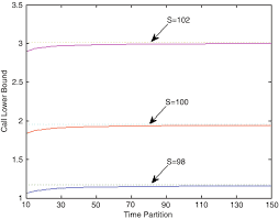
The SSD bounds (2.16) and (2.17) are distribution-free, recursive and applicable to any number of time partitions till option expiration. The question that arises, therefore, is their relationship with the continuous time option prices that have dominated option research in the more than 40 years since the BSM model first appeared. As it turns out, the two bounds converge to the same limit, the BSM model price, when the underlying asset returns follow diffusion asset dynamics. This was shown by Perrakis (1988) for a trinomial discretization of the continuous time distribution converging to lognormal diffusion and was generalized by Oancea and Perrakis (2014) for a general discretization converging to any type of diffusion.
We model the index return $z_{t+\Delta t}$ held by the trader in the equilibrium relations (2.1) in the following general form that guarantees convergence to diffusion as $\Delta t \rightarrow 0$
$$
z_{t+\Delta t}=\mu\left(S_t, t\right) \Delta t+\sigma\left(S_t, t\right) \varepsilon \sqrt{\Delta t} .
$$
In this expression $\varepsilon$ has a bounded distribution of mean zero and variance one, $\varepsilon \sim D(0,1)$ and $0<\varepsilon_{\min } \leq \varepsilon \leq \varepsilon_{\max }$, but otherwise unrestricted. In (2.26) the limit is the lognormal diffusion when the parameters $\mu$ and $\sigma$ are constant.
The discretization (2.26) can be easily shown to converge to diffusion. ${ }^{10}$ The main result of this section, however, is the convergence of the transformed return distributions that underlie the two option bounds. We use the weak convergence criterion for the two return processes. For any number $m$ of time periods to expiration, we define a sequence of stock prices $\left{S_t \mid \Delta t, m\right}$ and an associated probability measure $P^m$. The weak convergence property for such processes ${ }^{11}$ stipulates that for any continuous bounded function $f$ we must have $E^P\left[f\left(S_T^m\right)\right] \rightarrow E^P\left[f\left(S_T\right)\right]$, where the measure $P$ corresponds to diffusion limit of the process, to be defined shortly. $P_m$ is then said to converge weakly to $P$ and $S_T^m$ is said to converge in distribution to $S_T$. A necessary and sufficient condition for the convergence to a diffusion is the Lindeberg condition, which was used by Merton (1992) to develop criteria for the convergence of multinomial processes. In a general form, if $\phi_t$ denotes a discrete stochastic process in $d$-dimensional space, the Lindeberg condition states that a necessary and sufficient condition that $\phi_t$ converges weakly to a diffusion is that for any fixed $\delta>0$ we must have
$$
\lim {\Delta t \rightarrow 0} \frac{1}{\Delta t} \int{b+s} Q_{\Delta v}(\phi, d \varphi)=0
$$
where $Q_{\Delta t}(\phi, d \varphi)$ is the transition probability from $\phi_t=\phi$ to $\phi_{t+\Delta t}=\varphi$ during the time interval $\Delta t$. Intuitively, it requires that $\phi_t$ does not change very much when the time interval $\Delta t$ goes to zero.
期权理论代写
金融代写|期权定价理论代写Option Pricing Theory代考|SD Option Pricing by Pairwise Comparisons
从第一章回忆起 1 SSD 的基本属性是,对于每个代理人,效用函数必须是递增和凹的,这反过来意味着边际效 用函数是非递增的。此处将标的物和期权的投资者或交易者确定为决策者的这一基本属性是SD期权定价的方 法。在市场均衡模型中,这种边际效用被称为定价内核,是定义衍生资产均衡价格的基本要素。
我们考虑一个具有当前价格的标的资产的市场 $S_t$ 和每期回报率等于的无风险资产 $R$. 还有一个带有行使价的欧式 看涨期权 $K$ 在末来的某个时间到期 $T$. 时间最初假定为离散的 $t=0,1, \ldots, T$ ,具有长度间隔 $\Delta t$, 暗示 $R=e^{r \Delta t}=1+r \Delta t+o(\Delta t)$ ,在哪里 $r$ 表示伡续时间的利率。在每个区间内,标的资产都有回报 $\frac{S_{t+\Delta t}-S_t}{S_t} \equiv z_{t+\Delta t}$ ,其分布可能取决于 $S_t \cdot{ }^2$
除了微不足道的情况 $z_{t+\Delta t}$ 仅取两个值 指数市场在离散时间背景下是不完整的。在这样的市场中,期权的估值 不能产生唯一的价格。我们的市场均衡是根据以下足以得出结果的假设得出的:
经济中至少存在一个效用最大化的风险规避投资者(交易者),他只持有指数和无风险资产。 这个特定的投资者在期权市场上处于边缘地位。
无风险利率是非随机的。
金融代写|期权定价理论代写Option Pricing Theory代考|The FRICTIONLESS SD BoundS IN CONTINUOUS
SSD 边界 (2.16) 和 (2.17) 是无分布的、递归的并且适用于任意数量的时间分区直到期权到期。因此,出现的问 题是它们与自 BSM 模型首次出现以来 40 多年来主导期权研究的连续时间期权价格的关系。事实证明,当标的 资产收益遵循扩散资产动态时,这两个边界会收敛到相同的限制,即 BSM 模型价格。这由 Perrakis (1988) 证 明了连续时间分布的三项式离散化收敛于对数正态扩散,并被 Oancea 和 Perrakis (2014) 概括为收敛于任何类 型扩散的一般离散化。
我们对指数回报进行建模 $z_{t+\Delta t}$ 交易者在均衡关系 (2.1) 中持有以下一般形式,保证扩散收敛为 $\Delta t \rightarrow 0$
$$
z_{t+\Delta t}=\mu\left(S_t, t\right) \Delta t+\sigma\left(S_t, t\right) \varepsilon \sqrt{\Delta t} .
$$
在这个表达式中 $\varepsilon$ 具有均值零和方差一的有界分布, $\varepsilon \sim D(0,1)$ 和 $0<\varepsilon_{\min } \leq \varepsilon \leq \varepsilon_{\max }$ ,但除此之外不受限 制。在 (2.26) 中,极限是对数正态扩散,当参数 $\mu$ 和 $\sigma$ 是恒定的。 可以很容易地证明离散化 (2.26) 收敛于扩散。 ${ }^{10}$ 然而,本节的主要结果是作为两个期权边界基础的转换后收益 分布的收敛。我们对两个返回过程使用弱收敛准则。对于任何数字 $m$ 到到期的时间段,我们定义了一系列股票 我们必须有 $E^P\left[f\left(S_T^m\right)\right] \rightarrow E^P\left[f\left(S_T\right)\right]$, 其中测量 $P$ 对应于过程的扩散极限,即将定义。 $P_m$ 然后据说弱收 敛到 $P$ 和 $S_T^m$ 据说收敛于分布 $S_T$. 收敛到扩散的必要和充分条件是 Lindeberg 条件,Merton (1992) 使用该条件 来制定多项式过程收敛的标准。在一般形式下,如果 $\phi_t$ 表示一个离散随机过程 $d$-dimensional 空间, Lindeberg 条件指出一个充分必要条件 $\phi_t$ 弱收敛于扩散是对于任何固定的 $\delta>0$ 我们必须有
$$
\lim \Delta t \rightarrow 0 \frac{1}{\Delta t} \int b+s Q_{\Delta v}(\phi, d \varphi)=0
$$
在哪里 $Q_{\Delta t}(\phi, d \varphi)$ 是从 $\phi_t=\phi$ 至 $\phi_{t+\Delta t}=\varphi$ 在时间间隔内 $\Delta t$. 直觉上,它要求 $\phi_t$ 时间间隔变化不大 $\Delta t$ 归 零。

统计代写请认准statistics-lab™. statistics-lab™为您的留学生涯保驾护航。
金融工程代写
金融工程是使用数学技术来解决金融问题。金融工程使用计算机科学、统计学、经济学和应用数学领域的工具和知识来解决当前的金融问题,以及设计新的和创新的金融产品。
非参数统计代写
非参数统计指的是一种统计方法,其中不假设数据来自于由少数参数决定的规定模型;这种模型的例子包括正态分布模型和线性回归模型。
广义线性模型代考
广义线性模型(GLM)归属统计学领域,是一种应用灵活的线性回归模型。该模型允许因变量的偏差分布有除了正态分布之外的其它分布。
术语 广义线性模型(GLM)通常是指给定连续和/或分类预测因素的连续响应变量的常规线性回归模型。它包括多元线性回归,以及方差分析和方差分析(仅含固定效应)。
有限元方法代写
有限元方法(FEM)是一种流行的方法,用于数值解决工程和数学建模中出现的微分方程。典型的问题领域包括结构分析、传热、流体流动、质量运输和电磁势等传统领域。
有限元是一种通用的数值方法,用于解决两个或三个空间变量的偏微分方程(即一些边界值问题)。为了解决一个问题,有限元将一个大系统细分为更小、更简单的部分,称为有限元。这是通过在空间维度上的特定空间离散化来实现的,它是通过构建对象的网格来实现的:用于求解的数值域,它有有限数量的点。边界值问题的有限元方法表述最终导致一个代数方程组。该方法在域上对未知函数进行逼近。[1] 然后将模拟这些有限元的简单方程组合成一个更大的方程系统,以模拟整个问题。然后,有限元通过变化微积分使相关的误差函数最小化来逼近一个解决方案。
tatistics-lab作为专业的留学生服务机构,多年来已为美国、英国、加拿大、澳洲等留学热门地的学生提供专业的学术服务,包括但不限于Essay代写,Assignment代写,Dissertation代写,Report代写,小组作业代写,Proposal代写,Paper代写,Presentation代写,计算机作业代写,论文修改和润色,网课代做,exam代考等等。写作范围涵盖高中,本科,研究生等海外留学全阶段,辐射金融,经济学,会计学,审计学,管理学等全球99%专业科目。写作团队既有专业英语母语作者,也有海外名校硕博留学生,每位写作老师都拥有过硬的语言能力,专业的学科背景和学术写作经验。我们承诺100%原创,100%专业,100%准时,100%满意。
随机分析代写
随机微积分是数学的一个分支,对随机过程进行操作。它允许为随机过程的积分定义一个关于随机过程的一致的积分理论。这个领域是由日本数学家伊藤清在第二次世界大战期间创建并开始的。
时间序列分析代写
随机过程,是依赖于参数的一组随机变量的全体,参数通常是时间。 随机变量是随机现象的数量表现,其时间序列是一组按照时间发生先后顺序进行排列的数据点序列。通常一组时间序列的时间间隔为一恒定值(如1秒,5分钟,12小时,7天,1年),因此时间序列可以作为离散时间数据进行分析处理。研究时间序列数据的意义在于现实中,往往需要研究某个事物其随时间发展变化的规律。这就需要通过研究该事物过去发展的历史记录,以得到其自身发展的规律。
回归分析代写
多元回归分析渐进(Multiple Regression Analysis Asymptotics)属于计量经济学领域,主要是一种数学上的统计分析方法,可以分析复杂情况下各影响因素的数学关系,在自然科学、社会和经济学等多个领域内应用广泛。
MATLAB代写
MATLAB 是一种用于技术计算的高性能语言。它将计算、可视化和编程集成在一个易于使用的环境中,其中问题和解决方案以熟悉的数学符号表示。典型用途包括:数学和计算算法开发建模、仿真和原型制作数据分析、探索和可视化科学和工程图形应用程序开发,包括图形用户界面构建MATLAB 是一个交互式系统,其基本数据元素是一个不需要维度的数组。这使您可以解决许多技术计算问题,尤其是那些具有矩阵和向量公式的问题,而只需用 C 或 Fortran 等标量非交互式语言编写程序所需的时间的一小部分。MATLAB 名称代表矩阵实验室。MATLAB 最初的编写目的是提供对由 LINPACK 和 EISPACK 项目开发的矩阵软件的轻松访问,这两个项目共同代表了矩阵计算软件的最新技术。MATLAB 经过多年的发展,得到了许多用户的投入。在大学环境中,它是数学、工程和科学入门和高级课程的标准教学工具。在工业领域,MATLAB 是高效研究、开发和分析的首选工具。MATLAB 具有一系列称为工具箱的特定于应用程序的解决方案。对于大多数 MATLAB 用户来说非常重要,工具箱允许您学习和应用专业技术。工具箱是 MATLAB 函数(M 文件)的综合集合,可扩展 MATLAB 环境以解决特定类别的问题。可用工具箱的领域包括信号处理、控制系统、神经网络、模糊逻辑、小波、仿真等。