如果你也在 怎样代写抽样调查sampling theory of survey这个学科遇到相关的难题,请随时右上角联系我们的24/7代写客服。
抽样调查是一种非全面调查,根据随机的原则从总体中抽取部分实际数据进行调查,并运用概率估计方法,根据样本数据推算总体相应的数量指标的一种统计分析方法。
statistics-lab™ 为您的留学生涯保驾护航 在代写抽样调查sampling theory of survey方面已经树立了自己的口碑, 保证靠谱, 高质且原创的统计Statistics代写服务。我们的专家在代写抽样调查sampling theory of survey方面经验极为丰富,各种代写抽样调查sampling theory of survey相关的作业也就用不着说。
我们提供的抽样调查sampling theory of survey及其相关学科的代写,服务范围广, 其中包括但不限于:
- Statistical Inference 统计推断
- Statistical Computing 统计计算
- Advanced Probability Theory 高等楖率论
- Advanced Mathematical Statistics 高等数理统计学
- (Generalized) Linear Models 广义线性模型
- Statistical Machine Learning 统计机器学习
- Longitudinal Data Analysis 纵向数据分析
- Foundations of Data Science 数据科学基础
统计代写|抽样调查作业代写sampling theory of survey代考|Bayesian approach
Another inferential approach in survey sampling is Bayesian as we now discuss.
About $\mathrm{Y}=\left(y_1, \ldots, y_i, \ldots, y_N\right)$, let $\Omega=\left{\mathrm{Y} \mid\left(-\infty<a_i \leq y_i \leq b_i<+\infty\right)\right.$, with $a_i, b_i$ known or unknown $}$, called the universal parametric space. For a sample $s=\left(i_1, \ldots, i_n\right)$ and survey data $d=(s, y)=\left(\left(i_1, y_{i 1}\right), \ldots,\left(i_n, y_{i n}\right)\right)$, with $y=\left(y_{i 1}, \ldots, y_{i n}\right)$, let us write
$$
P{\mathrm{Y}}(d)=\operatorname{Prob}(d)=p(s) I{\mathrm{Y}}(d),
$$
where
$$
I_{Y}(d)=\left{\begin{array}{ll}
1 & \text { if } Y \in \Omega_d \
0 & \text { if } Y \notin \Omega_d
\end{array},\right.
$$
writing
$\Omega_d=\left{\mathrm{Y} \mid-\infty<a_j \leq y_j \leq b_j<\infty\right.$ for $j \neq i_1, \ldots, i_n$ but $y$ is as observed $}$, then we call $P_{\mathrm{Y}}(d)$, the probability of observing the survey data $d$ when $Y$ is in the underlying parametric space. A survey design $p$ is called ‘informative’ if $p(s)$ involves any element of $Y$ and it is called ‘non-informative’ in case $p(s)$ involves no element of $Y$. An informative design may be contemplated if, for example, sampling proceeds by choosing an element $i_1$, observing the $y_{i 1}$-value and allowing the value of $p\left(i_2 \mid\left(i_1, y_{i 1}\right)\right)$ to involve $y_{i 1}$ and likewise choosing successive elements in $s$ utilizing the $y$-values for the units already drawn in it. But, generally a design $p$ is ‘non-informative’. In case $p$ is non-informative, $\operatorname{Prob}(d)=p(s)$, which is a constant free of $Y$ so long as the underlying $Y$ belongs to $\Omega_d$ i.e. it is consistent with the observed survey data at hand. We take $P_{Y}(d)$ also as the ‘likelihood’ of $Y$ given the data $d$ and write it as
$$
L_d(\mathrm{Y})=P_{\mathrm{Y}}(d)=p(s) I_{\mathrm{Y}}(d) .
$$
Thus, for a ‘non-informative’ design, the likelihood is a constant, free of $Y$ so long as it involves $Y$ in $\Omega_d$; i.e. $Y$ is consistent with the data observed.
This flat likelihood in survey sampling is ‘sterile’ in inference-making concerning the variate-values yet unobserved for the sample at hand and already surveyed. This discussion is based on the classical works of Godambe (1966, 1969) and Basu (1969).
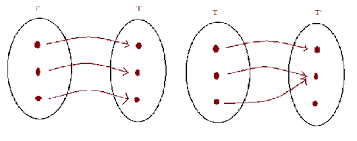
统计代写|抽样调查作业代写sampling theory of survey代考|Minimal sufficiency
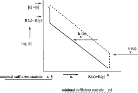
Just as $\zeta={s}$, the totality of all possible samples $s$ is the ‘sample space’, we shall call $D={d}$, the totality of all possible survey data points $d$ as the “data space”. This $D$ is the totality of all individual data points $d$. If a statistic $t=t(d)$ is defined, it has the effect of inducing on $D$ a ‘partitioning’. A partitioning creates a number of ‘partition sets’ of data points $d$ which are mutually disjoint and which together coincide with $D$. Two different statistics $t_1=t_1(d)$ and $t_2=t_2(d)$ generally induce two different partitionings on $D$. If every ‘partition set’ induced by $t_2$ is contained in a ‘partition set’ induced by $t_1$, then $t_1$ is said to induce a ‘thicker’ partitioning than $t_2$, which naturally induces a thinner partitioning. If both $t_1$ and $t_2$ are “sufficient”, then neither sacrifices any information of relevance and $t_1$ achieves more ‘summarization’ than $t_2$. So, one should prefer and work for a statistic which is sufficient and ‘induces the thickest partitioning’ and such a statistic is called the ‘Minimal Sufficient’ statistic which is the most desirable among all sufficient statistics.
Let $d_1$ and $d_2$ be two data points of the form $d$ and $d_1^, d_2^$ be two data points corresponding to them as $d^$ corresponds to $d$. Let $t=t($.$) be a sufficient$ statistic such that $t\left(d_1\right)=t\left(d_2\right)$. If we can show that this implies that $d_1^=d_2^$, then it will follow that $d^$ induces a thicker partitioning than $t$ implying that $d^$ is the ‘Minimal Sufficient’ statistic. We prove this below. Since $t$ is a sufficient statistic, $$ \begin{aligned} P_{Y}\left(d_1\right) & =P_{Y}\left(d_1 \cap t\left(d_1\right)\right) \ & -\Gamma_{Y}\left(t\left(d_1\right)\right) C_1 \text { with } C_1 \text { a constant; } \end{aligned} $$ since $t\left(d_1\right)=t\left(d_2\right)$ it follows that $$ \begin{aligned} P_{Y}\left(d_1\right) & =P{\mathbf{Y}}\left(t\left(d_1\right)\right) C_1=P{Y}\left(t\left(d_2\right)\right) C_2 \
& =P_{\mathbf{Y}}\left(d_2\right) \frac{C_1}{C_2}, \text { with } C_2 \text { a constant. }
\end{aligned}
$$
Since $d^$ is a sufficient statistic,
$P_{Y}\left(d_1^*\right)=P_{Y}\left(d_1\right) C_3, C_3$ is a constant.
抽样调查代考
统计代写|抽样调查作业代写sampling theory of survey代考|Bayesian approach
I_ ${Y}(d)=|$ left ${$ begin ${$ array $}{|}$
1 \& Itext ${$ if $} Y \backslash$ in $\backslash$ Omega_d $\backslash$
0 \& Itext ${$ if $} Y \backslash$ notin $\backslash 0$ mega_d lend{array}, \正确的。
$\$ \$$
写作
, theprobabilityofobservingthesurveydata $\mathrm{d}$ when 是
isintheunderlyingparametricspace. Asurveydesign iscalled $^*$ in formative if $^{\prime} \mathrm{p}(\mathrm{s})$
involvesanyelemento $f$ 是anditiscalled’non $-$ in formative’ incasep(s)
involvesnoelemento $f$ 是
. Aninformativedesignmaybecontemplatedif, forexample, samplingproceedsbychoosin i_1, observingthey_{i 1}-valueandallowingthevalueof $\mathrm{p} \backslash \mathrm{eft}(\mathrm{i} 2$ \mid \eft(i_1, y_{i
1}\right)\right)toinvolvey_{i 1}andlikewisechoosingsuccessiveelementsin 秒utilizingthe 是 -values fortheunitsalreadydrawninit. But, generallyadesign $\mathrm{p}$
is’non – informative’. Incasepisnon – informative, loperatorname ${$ 概率 $}(\mathrm{d})=\mathrm{p}(\mathrm{s})$
, whichisaconstantfreeo $f$ 是solongastheunderlying 是belongstolOmega_d
i.e.itisconsistentwiththeobservedsurveydataathand. Wetake $\mathrm{P}{-}{\mathrm{Y}}(\mathrm{d})$ alsoasthe ‘likelihood’of 是giventhedatadandwriteitas $\$$ $\mathrm{L}{-} \mathrm{d}(I m a t h r m{Y})=P_{-}{\operatorname{Imathrm}{\mathrm{Y}}}(\mathrm{d})=\mathrm{p}(\mathrm{s}) I_{-}{I m a t h r m{Y}}(\mathrm{d})$
$\$ \$$
因此,对于“非信息”设计,可能性是一个常数,不受 $\$$ Ysolongasitinvolves 是inlOmega_d; i.e.Y $\$$ 与 观察到的数据一致。
调查抽样中的这种平坦可能性在关于变量值的推断中是“无效的”,但对于手头和已经调查的样本尚末观察 到。此讨论基于 Godambe $(1966,1969)$ 和 Basu (1969) 的经典著作。
统计代写|抽样调查作业代写sampling theory of survey代考|Minimal sufficiency
正如 $\zeta=s$, 所有可能样本的总和 $s$ 是”样本空间”,我们称 $D=d$, 所有可能的调查数据点的总和 $d$ 作为 “数 据空间”。这个 $D$ 是所有单个数据点的总和 $d$. 如果统计 $t=t(d)$ 被定义,它具有谞导作用 $D$ 一个 “分区”。 分区会创建多个数据点的”分区集” $d$ 它们是相互不相交的,并且它们一起重合 $D$. 两种不同的统计 $t_1=t_1(d)$ 和 $t_2=t_2(d)$ 通常在 $D$. 如果每个”分区集”由 $t_2$ 包含在由 $t_1$ ,然后 $t_1$ 据说会导致比 $t_2$ ,这自然 会导致更薄的分区。如果两者 $t_1$ 和 $t_2$ 是 “足够的”,那么既不牺牲任何相关信息,又 $t_1$ 实现更多的“总结” $t_2$. 因此,人们应该更喜欢并为一个充分的统计量工作并”诱导最厚的划分”,这样的统计量被称为“最小充分”统 计量,它是所有充分统计量中最可取的。
让 $d_1$ 和 $d_2$ 是表格的两个数据点 $d$ 和 $\mathrm{d}{-} 1^{\wedge}, d{-} 2^{\wedge}$ 是对应于它们的两个数据点 $\wedge$ 对应于 $d$. 让 $t=t($. 导致比更厚的分区 $t$ 暗示 $\$ 是“最小足够”统计量。我们在下面证明这一点。自从 $t$ 是一个充分的统计量, $\$ \$$ }\eft(t\left(d_1\right)\right) C_1 \text { with } C_1 \text ${$ 一个常数; } 结束 ${$ 对齐 $}$
$$
\text { since } \$ t\left(d_1\right)=t\left(d_2\right) \text { \$itfollowsthat }
$$
Veft(d_2\right)\right) C_2\ lend{aligned $}$
$\$ \$$
因为 $\wedge$ 是充分统计量,
$\$ P_{-}{Y} \backslash$ left(d_1^*$\backslash$ right)=P_ ${Y} \backslash$ left(d_1\right) C_3,C_3\$是常数。

统计代写请认准statistics-lab™. statistics-lab™为您的留学生涯保驾护航。统计代写|python代写代考
随机过程代考
在概率论概念中,随机过程是随机变量的集合。 若一随机系统的样本点是随机函数,则称此函数为样本函数,这一随机系统全部样本函数的集合是一个随机过程。 实际应用中,样本函数的一般定义在时间域或者空间域。 随机过程的实例如股票和汇率的波动、语音信号、视频信号、体温的变化,随机运动如布朗运动、随机徘徊等等。
贝叶斯方法代考
贝叶斯统计概念及数据分析表示使用概率陈述回答有关未知参数的研究问题以及统计范式。后验分布包括关于参数的先验分布,和基于观测数据提供关于参数的信息似然模型。根据选择的先验分布和似然模型,后验分布可以解析或近似,例如,马尔科夫链蒙特卡罗 (MCMC) 方法之一。贝叶斯统计概念及数据分析使用后验分布来形成模型参数的各种摘要,包括点估计,如后验平均值、中位数、百分位数和称为可信区间的区间估计。此外,所有关于模型参数的统计检验都可以表示为基于估计后验分布的概率报表。
广义线性模型代考
广义线性模型(GLM)归属统计学领域,是一种应用灵活的线性回归模型。该模型允许因变量的偏差分布有除了正态分布之外的其它分布。
statistics-lab作为专业的留学生服务机构,多年来已为美国、英国、加拿大、澳洲等留学热门地的学生提供专业的学术服务,包括但不限于Essay代写,Assignment代写,Dissertation代写,Report代写,小组作业代写,Proposal代写,Paper代写,Presentation代写,计算机作业代写,论文修改和润色,网课代做,exam代考等等。写作范围涵盖高中,本科,研究生等海外留学全阶段,辐射金融,经济学,会计学,审计学,管理学等全球99%专业科目。写作团队既有专业英语母语作者,也有海外名校硕博留学生,每位写作老师都拥有过硬的语言能力,专业的学科背景和学术写作经验。我们承诺100%原创,100%专业,100%准时,100%满意。
机器学习代写
随着AI的大潮到来,Machine Learning逐渐成为一个新的学习热点。同时与传统CS相比,Machine Learning在其他领域也有着广泛的应用,因此这门学科成为不仅折磨CS专业同学的“小恶魔”,也是折磨生物、化学、统计等其他学科留学生的“大魔王”。学习Machine learning的一大绊脚石在于使用语言众多,跨学科范围广,所以学习起来尤其困难。但是不管你在学习Machine Learning时遇到任何难题,StudyGate专业导师团队都能为你轻松解决。
多元统计分析代考
基础数据: $N$ 个样本, $P$ 个变量数的单样本,组成的横列的数据表
变量定性: 分类和顺序;变量定量:数值
数学公式的角度分为: 因变量与自变量
时间序列分析代写
随机过程,是依赖于参数的一组随机变量的全体,参数通常是时间。 随机变量是随机现象的数量表现,其时间序列是一组按照时间发生先后顺序进行排列的数据点序列。通常一组时间序列的时间间隔为一恒定值(如1秒,5分钟,12小时,7天,1年),因此时间序列可以作为离散时间数据进行分析处理。研究时间序列数据的意义在于现实中,往往需要研究某个事物其随时间发展变化的规律。这就需要通过研究该事物过去发展的历史记录,以得到其自身发展的规律。
回归分析代写
多元回归分析渐进(Multiple Regression Analysis Asymptotics)属于计量经济学领域,主要是一种数学上的统计分析方法,可以分析复杂情况下各影响因素的数学关系,在自然科学、社会和经济学等多个领域内应用广泛。
MATLAB代写
MATLAB 是一种用于技术计算的高性能语言。它将计算、可视化和编程集成在一个易于使用的环境中,其中问题和解决方案以熟悉的数学符号表示。典型用途包括:数学和计算算法开发建模、仿真和原型制作数据分析、探索和可视化科学和工程图形应用程序开发,包括图形用户界面构建MATLAB 是一个交互式系统,其基本数据元素是一个不需要维度的数组。这使您可以解决许多技术计算问题,尤其是那些具有矩阵和向量公式的问题,而只需用 C 或 Fortran 等标量非交互式语言编写程序所需的时间的一小部分。MATLAB 名称代表矩阵实验室。MATLAB 最初的编写目的是提供对由 LINPACK 和 EISPACK 项目开发的矩阵软件的轻松访问,这两个项目共同代表了矩阵计算软件的最新技术。MATLAB 经过多年的发展,得到了许多用户的投入。在大学环境中,它是数学、工程和科学入门和高级课程的标准教学工具。在工业领域,MATLAB 是高效研究、开发和分析的首选工具。MATLAB 具有一系列称为工具箱的特定于应用程序的解决方案。对于大多数 MATLAB 用户来说非常重要,工具箱允许您学习和应用专业技术。工具箱是 MATLAB 函数(M 文件)的综合集合,可扩展 MATLAB 环境以解决特定类别的问题。可用工具箱的领域包括信号处理、控制系统、神经网络、模糊逻辑、小波、仿真等。