如果你也在 怎样代写嵌入式软件Embedded Software这个学科遇到相关的难题，请随时右上角联系我们的24/7代写客服。

嵌入式软件是指人类用户不能直接看到或调用的软件，但它是系统的一部分。例如，软件被嵌入到电视机、飞机和电子游戏中。嵌入式软件被用来控制硬件设备的功能。

statistics-lab™ 为您的留学生涯保驾护航 在代写嵌入式软件Embedded Software方面已经树立了自己的口碑, 保证靠谱, 高质且原创的统计Statistics代写服务。我们的专家在代写嵌入式软件Embedded Software代写方面经验极为丰富，各种代写嵌入式软件Embedded Software相关的作业也就用不着说。

我们提供的嵌入式软件Embedded Software及其相关学科的代写，服务范围广, 其中包括但不限于:

• Statistical Inference 统计推断
• Statistical Computing 统计计算
• Advanced Probability Theory 高等概率论
• Advanced Mathematical Statistics 高等数理统计学
• (Generalized) Linear Models 广义线性模型
• Statistical Machine Learning 统计机器学习
• Longitudinal Data Analysis 纵向数据分析
• Foundations of Data Science 数据科学基础

计算机代写|嵌入式软件代写Embedded Software代考|Wait States and Burst Accesses

There are a variety of different types of storage, all of which have their advantages and disadvantages. RAM is fast as well as readable and writable, but is said to be volatile as it loses its contents if not permanently powered. Flash is persistent memory (non-volatile) but access to it is relatively slow. In most cases it is so slow that access to it must be artificially slowed down. This is achieved by using ‘wait states’ for each access during which the processor waits for the memory to respond.
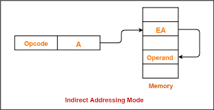
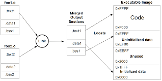
As discussed in detail in Section 2.3, each time memory is accessed, the address to be accessed must be specified. With respect to the transfer of user data, the exchange of address information can be seen as a kind of overhead (Figure 7). During the execution of code, several memory locations are very often read in sequence, especially whenever there are no jumps or function calls (keyword: basic block). The same applies to the initialization of variables with values from the flash: the values are often stored in memory one after the other.

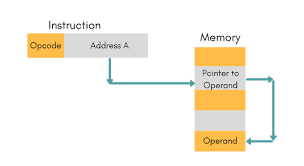
In both cases there would be many individual read accesses, each with significant overhead (Figure 8). To make this type of access more efficient, many memories offer burst accesses. These can transfer an entire range of data starting from a single address (Figure 9), significantly reducing the overhead.

In a tax office, a clerk deals with the affairs of four clients in one morning. Her files are put on the desk for quick access. After all, she has to look at individual documents again and again and does not want to fetch the file from the archive for each document and then return the file back to the archive after viewing it. That would be inefficient.

This office procedure describes the concept of a cache very well. A comparatively small but very fast memory (desktop equates to cache) is loaded with the current contents of a much larger, but also much slower, memory (archive equates to flash or shared RAM), as in Figure 10.

With larger processors, further gradations or cache levels come into play. The example of the tax office could be extended as follows to illustrate multi-level caches. Between the desk and the archive there may also be a drawer unit on castors under the desk, as well as a filing cabinet in the office. This results in the following gradation: desk equates to level 1 cache, hanging file register equates to level 2 cache, filing cabinet equates to level 3 cache, and finally archive equals flash or shared RAM. Usually the word ‘level’ is not written out in full but simply replaced by an ‘ $L$ ‘. Thus we speak of an $\mathrm{L} 1$ cache, $\mathrm{L} 2$ cache and so on.

If data or code is to be read and it is already in the cache, this is called a cache hit. If they are not in the cache and must first be fetched from main memory, there is a cache miss.

计算机代写|嵌入式软件代写Embedded Software代考|Cache Structure and Cache Rows

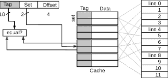
Each cache is divided into cache lines, each line being several dozen bytes in size. The main memory is an integer multiple larger than the cache, so the cache fits in ‘ $n$ times’. When transferring data to or from the cache, an entire cache line is always transferred by burst access.

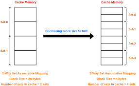
The assignment of cache lines to the memory addresses in the main memory is not freely selectable. Instead, it results from the position of the line in the cache. Figure 11 illustrates the relationship. Cache line 3 , for example, can only be matched with memory areas marked with a ‘ 3 ‘. In reality, the size ratio is more pronounced than the 1:4 ratio used in the figure and the number of cache lines is also significantly higher. Table 2 shows the parameters as they are defined for first generation Infineon AURIX processors.

To illustrate how the cache works, let us assume a concrete situation in which a function FunctionA has already been loaded into a cache line (Figure 12). Obviously, the function is small enough to fit completely into a cache line. Three different cases will be considered below.

What happens if the cached function FunctionA now calls: (I) the function FunctionB; (II) the function Functionc; or (III) the function FunctionA (i.e. recursively calls itself)?
(I) Function FunctionB is loaded into cache line 3 and thus overwrites Functiona.
(II) Function Functione is loaded into cache line 4 and FunctionA remains in cache line 3.
(III) Nothing happens because FunctionA is already in cache line 3 .

嵌入式软件代考

计算机代写|嵌入式软件代写Embedded Software代考|Wait States and Burst Accesses

有多种不同类型的存储，它们各有优缺点。RAM 速度快，可读可写，但据说是易失性的，因为如果不永久供电，它会丢失其内容。闪存是持久性内存（非易失性），但访问速度相对较慢。在大多数情况下，它是如此之慢，以至于必须人为地减慢对它的访问。这是通过对处理器等待内存响应的每次访问使用“等待状态”来实现的。
正如 2.3 节中详细讨论的那样，每次访问内存时，都必须指定要访问的地址。对于用户数据的传输，地址信息的交换可以看作是一种开销（图 7）。在代码执行过程中，通常会依次读取多个内存位置，尤其是在没有跳转或函数调用（关键字：基本块）的情况下。这同样适用于使用闪存中的值初始化变量：这些值通常一个接一个地存储在内存中。

在这两种情况下，都会有许多单独的读取访问，每个读取访问都有很大的开销（图 8）。为了使这种类型的访问更有效，许多存储器提供突发访问。这些可以从单个地址开始传输整个范围的数据（图 9），从而显着减少开销。

在一家税务局，一名文员一天要处理四位客户的事务。她的文件放在桌子上以便快速访问。毕竟，她不得不一次又一次地查看单个文档，并且不想为每个文档从存档中获取文件，然后在查看后将文件返回到存档中。那将是低效的。

这个办公程序很好地描述了缓存的概念。一个相对较小但速度非常快的内存（桌面相当于缓存）加载了一个更大但也更慢的内存（归档相当于闪存或共享 RAM）的当前内容，如图 10 所示。

使用更大的处理器，更多的层次或缓存级别开始发挥作用。税务局的示例可以扩展如下，以说明多级缓存。在办公桌和档案室之间，办公桌下方的脚轮上可能还有一个抽屉单元，办公室中还有一个文件柜。这导致以下分级：书桌等同于 1 级缓存，悬挂文件寄存器等同于 2 级缓存，文件柜等同于 3 级缓存，最后档案等同于闪存或共享 RAM。通常“级别”这个词没有写完整，而只是简单地用一个“大号’. 因此我们谈到一个大号1缓存，大号2缓存等。

如果要读取的数据或代码已经在缓存中，则称为缓存命中。如果它们不在高速缓存中并且必须首先从主存中获取，则存在高速缓存未命中。

计算机代写|嵌入式软件代写Embedded Software代考|Cache Structure and Cache Rows

每个缓存被分成缓存行，每行大小为几十个字节。主内存比缓存大一个整数倍，所以缓存适合’n次’。当向高速缓存传输数据或从高速缓存传输数据时，整个高速缓存行总是通过突发访问传输。

高速缓存线到主存储器中存储器地址的分配不是可以自由选择的。相反，它是由行在缓存中的位置产生的。图 11 说明了这种关系。例如，缓存行 3 只能与标有“ 3 ”的内存区域匹配。实际上，大小比例比图中使用的 1:4 比例更明显，缓存行数也明显更高。表 2 显示了为第一代英飞凌 AURIX 处理器定义的参数。

为了说明缓存的工作原理，让我们假设一个具体情况，其中函数 FunctionA 已经加载到缓存行中（图 12）。显然，该函数足够小，可以完全放入缓存行中。下面将考虑三种不同的情况。

如果缓存函数 FunctionA 现在调用： (I) 函数 FunctionB；(II)函数Functionc；或 (III) 函数 FunctionA（即递归调用自身）？
(I) 函数 FunctionB 被加载到缓存行 3 并因此覆盖 Functiona。
(II) 函数 Functione 被加载到缓存行 4 中，而 FunctionA 保留在缓存行 3 中。
(III) 什么都没有发生，因为 FunctionA 已经在缓存行 3 中。

统计代写请认准statistics-lab™. statistics-lab™为您的留学生涯保驾护航。

金融工程代写

金融工程是使用数学技术来解决金融问题。金融工程使用计算机科学、统计学、经济学和应用数学领域的工具和知识来解决当前的金融问题，以及设计新的和创新的金融产品。

非参数统计代写

非参数统计指的是一种统计方法，其中不假设数据来自于由少数参数决定的规定模型；这种模型的例子包括正态分布模型和线性回归模型。

广义线性模型代考

广义线性模型（GLM）归属统计学领域，是一种应用灵活的线性回归模型。该模型允许因变量的偏差分布有除了正态分布之外的其它分布。

术语 广义线性模型（GLM）通常是指给定连续和/或分类预测因素的连续响应变量的常规线性回归模型。它包括多元线性回归，以及方差分析和方差分析（仅含固定效应）。

有限元方法代写

有限元方法（FEM）是一种流行的方法，用于数值解决工程和数学建模中出现的微分方程。典型的问题领域包括结构分析、传热、流体流动、质量运输和电磁势等传统领域。

有限元是一种通用的数值方法，用于解决两个或三个空间变量的偏微分方程（即一些边界值问题）。为了解决一个问题，有限元将一个大系统细分为更小、更简单的部分，称为有限元。这是通过在空间维度上的特定空间离散化来实现的，它是通过构建对象的网格来实现的：用于求解的数值域，它有有限数量的点。边界值问题的有限元方法表述最终导致一个代数方程组。该方法在域上对未知函数进行逼近。[1] 然后将模拟这些有限元的简单方程组合成一个更大的方程系统，以模拟整个问题。然后，有限元通过变化微积分使相关的误差函数最小化来逼近一个解决方案。

tatistics-lab作为专业的留学生服务机构，多年来已为美国、英国、加拿大、澳洲等留学热门地的学生提供专业的学术服务，包括但不限于Essay代写，Assignment代写，Dissertation代写，Report代写，小组作业代写，Proposal代写，Paper代写，Presentation代写，计算机作业代写，论文修改和润色，网课代做，exam代考等等。写作范围涵盖高中，本科，研究生等海外留学全阶段，辐射金融，经济学，会计学，审计学，管理学等全球99%专业科目。写作团队既有专业英语母语作者，也有海外名校硕博留学生，每位写作老师都拥有过硬的语言能力，专业的学科背景和学术写作经验。我们承诺100%原创，100%专业，100%准时，100%满意。

随机分析代写

随机微积分是数学的一个分支，对随机过程进行操作。它允许为随机过程的积分定义一个关于随机过程的一致的积分理论。这个领域是由日本数学家伊藤清在第二次世界大战期间创建并开始的。

时间序列分析代写

随机过程，是依赖于参数的一组随机变量的全体，参数通常是时间。 随机变量是随机现象的数量表现，其时间序列是一组按照时间发生先后顺序进行排列的数据点序列。通常一组时间序列的时间间隔为一恒定值（如1秒，5分钟，12小时，7天，1年），因此时间序列可以作为离散时间数据进行分析处理。研究时间序列数据的意义在于现实中，往往需要研究某个事物其随时间发展变化的规律。这就需要通过研究该事物过去发展的历史记录，以得到其自身发展的规律。

回归分析代写

多元回归分析渐进（Multiple Regression Analysis Asymptotics）属于计量经济学领域，主要是一种数学上的统计分析方法，可以分析复杂情况下各影响因素的数学关系，在自然科学、社会和经济学等多个领域内应用广泛。

MATLAB代写

MATLAB 是一种用于技术计算的高性能语言。它将计算、可视化和编程集成在一个易于使用的环境中，其中问题和解决方案以熟悉的数学符号表示。典型用途包括：数学和计算算法开发建模、仿真和原型制作数据分析、探索和可视化科学和工程图形应用程序开发，包括图形用户界面构建MATLAB 是一个交互式系统，其基本数据元素是一个不需要维度的数组。这使您可以解决许多技术计算问题，尤其是那些具有矩阵和向量公式的问题，而只需用 C 或 Fortran 等标量非交互式语言编写程序所需的时间的一小部分。MATLAB 名称代表矩阵实验室。MATLAB 最初的编写目的是提供对由 LINPACK 和 EISPACK 项目开发的矩阵软件的轻松访问，这两个项目共同代表了矩阵计算软件的最新技术。MATLAB 经过多年的发展，得到了许多用户的投入。在大学环境中，它是数学、工程和科学入门和高级课程的标准教学工具。在工业领域，MATLAB 是高效研究、开发和分析的首选工具。MATLAB 具有一系列称为工具箱的特定于应用程序的解决方案。对于大多数 MATLAB 用户来说非常重要，工具箱允许您学习和应用专业技术。工具箱是 MATLAB 函数（M 文件）的综合集合，可扩展 MATLAB 环境以解决特定类别的问题。可用工具箱的领域包括信号处理、控制系统、神经网络、模糊逻辑、小波、仿真等。

R语言代写	问卷设计与分析代写
PYTHON代写	回归分析与线性模型代写
MATLAB代写	方差分析与试验设计代写
STATA代写	机器学习/统计学习代写
SPSS代写	计量经济学代写
EVIEWS代写	时间序列分析代写
EXCEL代写	深度学习代写
SQL代写	各种数据建模与可视化代写

如果你也在 怎样代写嵌入式软件Embedded Software这个学科遇到相关的难题，请随时右上角联系我们的24/7代写客服。

嵌入式软件是指人类用户不能直接看到或调用的软件，但它是系统的一部分。例如，软件被嵌入到电视机、飞机和电子游戏中。嵌入式软件被用来控制硬件设备的功能。

statistics-lab™ 为您的留学生涯保驾护航 在代写嵌入式软件Embedded Software方面已经树立了自己的口碑, 保证靠谱, 高质且原创的统计Statistics代写服务。我们的专家在代写嵌入式软件Embedded Software代写方面经验极为丰富，各种代写嵌入式软件Embedded Software相关的作业也就用不着说。

我们提供的嵌入式软件Embedded Software及其相关学科的代写，服务范围广, 其中包括但不限于:

• Statistical Inference 统计推断
• Statistical Computing 统计计算
• Advanced Probability Theory 高等概率论
• Advanced Mathematical Statistics 高等数理统计学
• (Generalized) Linear Models 广义线性模型
• Statistical Machine Learning 统计机器学习
• Longitudinal Data Analysis 纵向数据分析
• Foundations of Data Science 数据科学基础

计算机代写|嵌入式软件代写Embedded Software代考|Code Execution

Section $1.3$ explained how the executable machine code is generated and that this code is a collection of machine instructions. The computational core of a microprocessor is constantly processing machine instructions. These instructions are loaded sequentially from program memory (or code memory) into the execution unit, whereupon they are decoded and then executed.

The program counter (PC) has already been mentioned, and it can be thought of as pointing to the current command in the program memory. As long as there are no jump commands or commands calling a (sub-)function, the PC is increased by one memory location once the processing of a command is complete. As a result, the PC points to the next command, which in turn is loaded into the execution unit, and then decoded and executed. The program memory is primarily a sequence of machine commands.

At this point it should be mentioned that a series of machine commands without any jump or call is referred to as a basic block. More precisely, a basic block is a series of machine instructions whose execution always starts with the first instruction, then sequentially executes all its instructions and terminates with the execution of the last instruction. The processor does not jump into, or out of, the basic block at any other point than its first or last instruction respectively. Basic blocks play an important role, amongst other things, in static code analysis, so we will return to this topic later.

The instructions provided by a processor are described in the processor’s Instruction Set Reference Manual. Knowledge of the instruction set of a processor is essential for optimizing software at the code level. Section $8.3$ will cover this in detail.

How an instruction set is documented, coded, and handled will be illustrated using the example of an add instruction on the 8-bit Microchip AVR processor. Microchip AVR processors have 32 data/address registers. Their role as data register or address register depends on the instruction. Figure 5 shows an excerpt (a single page) from the instruction set reference manual for the Microchip AVR ATmega processor [3], namely the section that describes the add command with carry flag. The description in textual and operational form $(R d \leftarrow R d+R r+C)$ is followed by the definition of the syntax.

计算机代写|嵌入式软件代写Embedded Software代考|Memory Addressing and Addressing Modes

The addressing mode describes how the memory is accessed. Each memory access requires the definition of the address to access as well as what should be done with the data at that address. This could range from using it to store data at the address, read from it, jump to it, call a subroutine at this address, and so on.

For runtime optimization at the code level, it is essential to know the addressing modes of the respective processor. Most processor architecture manuals (often part of the instruction reference manual) have a section that describes the available addressing modes in detail.

As the previous Section $2.2$ showed, the opcode defines what should happen, such as ‘continue program execution at address x’ (a jump command), or ‘load the contents of address y into working register $\mathrm{d} 4$ ‘. The address to which some action should occur is passed as a parameter. On a 32-bit processor, the address bus has a width of 32 bits. Almost all processors are designed so that there is one byte of memory for each address. Thus $2^{32}=4,294,967,296$ single bytes can be addressed, which corresponds to 4 gigabytes. Strictly speaking, according to the IEC [4] it should be called 4 gibibytes because the prefix giga stands for $10^9$ and not for $2^{30}$. In practice, however, the prefixes kibi $\left(2^{10}\right)$, mebi $\left(2^{20}\right)$, gibi $\left(2^{30}\right)$, tebi $\left(2^{40}\right)$ etc., which are based on powers of two, are hardly ever used. For this reason, we will also talk about kilobytes and megabytes in the following when referring to $2^{10}$ or $2^{20}$ bytes respectively.

But back to the 4-gigabyte address space. Most embedded systems, even those with 32-bit processors, have much smaller quantities of memory, typically ranging from a few kilobytes to a few megabytes.

If 32 -bit addresses were always used this would be very inefficient as, for each memory access, the opcode as well as the full 32-bit address would have to be loaded. For this reason, all processors offer a range of addressing modes in addition to far addressing, the name given to the use of the full address bus width.

It is difficult to describe all existing types of addressing comprehensively and it is not useful at this point. Instead, some examples will be picked out for certain processors that differ in their implementation from the description here or have special features. Additionally, processor manufacturers have come up with a number of special addressing types that are not discussed here. For the following explanation of addressing types a fictive 16-bit processor is used. It has 64 kilobytes of program memory (flash) and 64 kilobytes of data memory (RAM). It also has eight data registers $R 0 \ldots R 7$ and eight address registers $A 0 \ldots A 7$. With each clock cycle, the CPU reads one word, i.e. 16 bits, from the program memory.

嵌入式软件代考

计算机代写|嵌入式软件代写Embedded Software代考|Code Execution

部分1.3解释了可执行机器代码是如何生成的，并且该代码是机器指令的集合。微处理器的计算核心不断处理机器指令。这些指令顺序地从程序存储器（或代码存储器）加载到执行单元中，随后它们被解码然后被执行。

程序计数器（PC）前面已经提到了，它可以认为是指向程序存储器中的当前命令。只要没有跳转命令或调用（子）函数的命令，一旦命令处理完成，PC 就会增加一个内存位置。结果，PC 指向下一条命令，这条命令又被加载到执行单元中，然后解码并执行。程序存储器主要是一系列机器命令。

这里需要说明的是，一系列没有任何跳转或调用的机器指令称为一个基本块。更准确地说，基本块是一系列机器指令，其执行总是从第一条指令开始，然后依次执行其所有指令，并以最后一条指令的执行结束。处理器不会分别在第一条或最后一条指令之外的任何其他点跳入或跳出基本块。基本块在静态代码分析中起着重要的作用，因此我们稍后会回到这个主题。

处理器提供的指令在处理器的指令集参考手册中进行了描述。处理器指令集的知识对于在代码级别优化软件至关重要。部分8.3将详细介绍这一点。

将使用 8 位 Microchip AVR 处理器上的加法指令示例说明如何记录、编码和处理指令集。Microchip AVR 处理器有 32 个数据/地址寄存器。它们作为数据寄存器或地址寄存器的作用取决于指令。图 5 显示了 Microchip AVR ATmega 处理器 [3] 指令集参考手册的摘录（单页），即描述带有进位标志的加法命令的部分。文字和操作形式的描述(Rd←Rd+Rr+C)后面是语法的定义。

计算机代写|嵌入式软件代写Embedded Software代考|Memory Addressing and Addressing Modes

寻址方式描述了内存是如何被访问的。每次内存访问都需要定义要访问的地址以及应该如何处理该地址的数据。这可能包括使用它在该地址存储数据、从中读取数据、跳转到该地址、在该地址调用子程序等等。

对于代码级别的运行时优化，了解各个处理器的寻址模式至关重要。大多数处理器体系结构手册（通常是指令参考手册的一部分）都有一个部分详细描述了可用的寻址模式。

正如上一节2.2显示，操作码定义了应该发生什么，例如“在地址 x 处继续程序执行”（跳转命令），或“将地址 y 的内容加载到工作寄存器中”d4′. 应该发生某些动作的地址作为参数传递。在 32 位处理器上，地址总线的宽度为 32 位。几乎所有的处理器都被设计成每个地址都有一个字节的内存。因此232=4,294,967,296可以寻址单个字节，相当于 4 GB。严格来说，根据 IEC [4]，它应该被称为 4 gibibytes，因为前缀 giga 代表109而不是为了230. 然而，在实践中，前缀 kibi(210)， 或许(220)， 喜欢(230)， 给你(240)等等，这是基于二的权力，几乎从未使用过。为此，我们在后面提到千字节和兆字节的时候也会说到210或者220字节分别。

但回到 4 GB 地址空间。大多数嵌入式系统，即使是那些带有 32 位处理器的系统，内存量也要小得多，通常从几千字节到几兆字节不等。

如果始终使用 32 位地址，这将非常低效，因为对于每次内存访问，都必须加载操作码以及完整的 32 位地址。出于这个原因，除了远寻址之外，所有处理器都提供了一系列寻址模式，远寻址是使用全地址总线宽度的名称。

很难全面地描述所有现有的寻址类型，并且在这一点上没有用处。相反，将为某些处理器挑选一些示例，这些处理器的实现与此处的描述不同或具有特殊功能。此外，处理器制造商提出了许多此处未讨论的特殊寻址类型。对于以下寻址类型的解释，使用了一个虚构的 16 位处理器。它有 64 KB 的程序存储器（闪存）和 64 KB 的数据存储器（RAM）。它还具有八个数据寄存器R0…R7和八个地址寄存器A0…A7. 在每个时钟周期，CPU 从程序存储器中读取一个字，即 16 位。

统计代写请认准statistics-lab™. statistics-lab™为您的留学生涯保驾护航。

金融工程代写

金融工程是使用数学技术来解决金融问题。金融工程使用计算机科学、统计学、经济学和应用数学领域的工具和知识来解决当前的金融问题，以及设计新的和创新的金融产品。

非参数统计代写

非参数统计指的是一种统计方法，其中不假设数据来自于由少数参数决定的规定模型；这种模型的例子包括正态分布模型和线性回归模型。

广义线性模型代考

广义线性模型（GLM）归属统计学领域，是一种应用灵活的线性回归模型。该模型允许因变量的偏差分布有除了正态分布之外的其它分布。

术语 广义线性模型（GLM）通常是指给定连续和/或分类预测因素的连续响应变量的常规线性回归模型。它包括多元线性回归，以及方差分析和方差分析（仅含固定效应）。

有限元方法代写

有限元方法（FEM）是一种流行的方法，用于数值解决工程和数学建模中出现的微分方程。典型的问题领域包括结构分析、传热、流体流动、质量运输和电磁势等传统领域。

有限元是一种通用的数值方法，用于解决两个或三个空间变量的偏微分方程（即一些边界值问题）。为了解决一个问题，有限元将一个大系统细分为更小、更简单的部分，称为有限元。这是通过在空间维度上的特定空间离散化来实现的，它是通过构建对象的网格来实现的：用于求解的数值域，它有有限数量的点。边界值问题的有限元方法表述最终导致一个代数方程组。该方法在域上对未知函数进行逼近。[1] 然后将模拟这些有限元的简单方程组合成一个更大的方程系统，以模拟整个问题。然后，有限元通过变化微积分使相关的误差函数最小化来逼近一个解决方案。

tatistics-lab作为专业的留学生服务机构，多年来已为美国、英国、加拿大、澳洲等留学热门地的学生提供专业的学术服务，包括但不限于Essay代写，Assignment代写，Dissertation代写，Report代写，小组作业代写，Proposal代写，Paper代写，Presentation代写，计算机作业代写，论文修改和润色，网课代做，exam代考等等。写作范围涵盖高中，本科，研究生等海外留学全阶段，辐射金融，经济学，会计学，审计学，管理学等全球99%专业科目。写作团队既有专业英语母语作者，也有海外名校硕博留学生，每位写作老师都拥有过硬的语言能力，专业的学科背景和学术写作经验。我们承诺100%原创，100%专业，100%准时，100%满意。

随机分析代写

随机微积分是数学的一个分支，对随机过程进行操作。它允许为随机过程的积分定义一个关于随机过程的一致的积分理论。这个领域是由日本数学家伊藤清在第二次世界大战期间创建并开始的。

时间序列分析代写

随机过程，是依赖于参数的一组随机变量的全体，参数通常是时间。 随机变量是随机现象的数量表现，其时间序列是一组按照时间发生先后顺序进行排列的数据点序列。通常一组时间序列的时间间隔为一恒定值（如1秒，5分钟，12小时，7天，1年），因此时间序列可以作为离散时间数据进行分析处理。研究时间序列数据的意义在于现实中，往往需要研究某个事物其随时间发展变化的规律。这就需要通过研究该事物过去发展的历史记录，以得到其自身发展的规律。

回归分析代写

多元回归分析渐进（Multiple Regression Analysis Asymptotics）属于计量经济学领域，主要是一种数学上的统计分析方法，可以分析复杂情况下各影响因素的数学关系，在自然科学、社会和经济学等多个领域内应用广泛。

MATLAB代写

MATLAB 是一种用于技术计算的高性能语言。它将计算、可视化和编程集成在一个易于使用的环境中，其中问题和解决方案以熟悉的数学符号表示。典型用途包括：数学和计算算法开发建模、仿真和原型制作数据分析、探索和可视化科学和工程图形应用程序开发，包括图形用户界面构建MATLAB 是一个交互式系统，其基本数据元素是一个不需要维度的数组。这使您可以解决许多技术计算问题，尤其是那些具有矩阵和向量公式的问题，而只需用 C 或 Fortran 等标量非交互式语言编写程序所需的时间的一小部分。MATLAB 名称代表矩阵实验室。MATLAB 最初的编写目的是提供对由 LINPACK 和 EISPACK 项目开发的矩阵软件的轻松访问，这两个项目共同代表了矩阵计算软件的最新技术。MATLAB 经过多年的发展，得到了许多用户的投入。在大学环境中，它是数学、工程和科学入门和高级课程的标准教学工具。在工业领域，MATLAB 是高效研究、开发和分析的首选工具。MATLAB 具有一系列称为工具箱的特定于应用程序的解决方案。对于大多数 MATLAB 用户来说非常重要，工具箱允许您学习和应用专业技术。工具箱是 MATLAB 函数（M 文件）的综合集合，可扩展 MATLAB 环境以解决特定类别的问题。可用工具箱的领域包括信号处理、控制系统、神经网络、模糊逻辑、小波、仿真等。

R语言代写	问卷设计与分析代写
PYTHON代写	回归分析与线性模型代写
MATLAB代写	方差分析与试验设计代写
STATA代写	机器学习/统计学习代写
SPSS代写	计量经济学代写
EVIEWS代写	时间序列分析代写
EXCEL代写	深度学习代写
SQL代写	各种数据建模与可视化代写

如果你也在 怎样代写嵌入式软件Embedded Software这个学科遇到相关的难题，请随时右上角联系我们的24/7代写客服。

嵌入式软件是指人类用户不能直接看到或调用的软件，但它是系统的一部分。例如，软件被嵌入到电视机、飞机和电子游戏中。嵌入式软件被用来控制硬件设备的功能。

statistics-lab™ 为您的留学生涯保驾护航 在代写嵌入式软件Embedded Software方面已经树立了自己的口碑, 保证靠谱, 高质且原创的统计Statistics代写服务。我们的专家在代写嵌入式软件Embedded Software代写方面经验极为丰富，各种代写嵌入式软件Embedded Software相关的作业也就用不着说。

我们提供的嵌入式软件Embedded Software及其相关学科的代写，服务范围广, 其中包括但不限于:

• Statistical Inference 统计推断
• Statistical Computing 统计计算
• Advanced Probability Theory 高等概率论
• Advanced Mathematical Statistics 高等数理统计学
• (Generalized) Linear Models 广义线性模型
• Statistical Machine Learning 统计机器学习
• Longitudinal Data Analysis 纵向数据分析
• Foundations of Data Science 数据科学基础

计算机代写|嵌入式软件代写Embedded Software代考|Phase Driven Process Model: The V-Model

The V-model describes a concept to approach software development. It has been used for decades in the automotive industry and is usually also available – at least in the background – when newer concepts, such as Scrum, are being developed. Like so many technical developments it has its origin in the military sector. Later, it was transferred to the civilian sector and was adapted to new development requirements in the versions V-Model 97 and V-Model XT[1].

The ‘ $\mathrm{V}$ ‘ of the $\mathrm{V}$-model represents the idealized course of development in a coordinate system with two axes. The horizontal axis is a time axis with the left side marking the project start. The vertical axis describes the level of abstraction, from ‘detailed’ at the bottom to ‘abstract’ at the top (Figure 1). A project should start at a high level of abstraction with a collection of user or customer requirements for the product. This is followed by the basic design of the product at system level. Over the course of the project the design is then broken down, refined, and improved. Additional, more detailed requirements may also emerge later. Once the design phase is complete, the implementation phase begins. With respect to a software project, this corresponds to the coding. Individual components are brought together at the integration phase, and this is followed by the verification, checking the fulfillment of the requirements at the different levels of abstraction. The final phase of validation takes place at the highest level of abstraction by ensuring that the user or customer requirements are met.

If a requirement is not fulfilled, the cause of the deviation must be eliminated. The cause is inevitably somewhere on the $\mathrm{V}$ between the requirement and its verification. As a result, all subsequent dependent steps must also be corrected, adapted, or at least repeated.

It is clear that the effort and associated cost to resolve an issue will grow depending on how late that issue is discovered. This reads like a truism, but it is astonishing how many projects completely neglect embedded software timing. Far too often, runtime problems are investigated in a late project phase with lots of hectic, high costs and risk, only for them to be temporarily corrected or mitigated.

计算机代写|嵌入式软件代写Embedded Software代考|Linker Script

The linker script (or linker control file) also plays a very important role. Strictly speaking, it should be called the ‘locator script’ or ‘locator control file’ but, as mentioned earlier, most vendors combine the locator into the linker.

Listing 5 shows an excerpt of the linker script of an 8-bit microcontroller, the Microchip AVR ATmega32, that has 32 KByte flash, 2 KByte RAM, and 1 KByte EEPROM.

The linker script tells the locator how to distribute the symbols across the different memory regions of the microcontroller. This is usually done as follows. First, in the $\mathrm{C}$ or assembler source code, all symbols are assigned to a specific section or, more precisely, a specific input section. This assignment will be made implicitly if the programmer has not made them explicitly. The following section names have become commonplace, representing default sections.

It is also an unwritten rule that section names begin with a dot.
In the step that follows, the instructions in the linker script assign all input sections to output sections which, in turn, are finally mapped to the available memory. For a better understanding, the .text sections in the Listing 5 have corresponding comments.

In a classic linker script, as in Listing 5, the definitions of the available memory are at the beginning. These are followed by the definitions of the output sections and, with each of these definitions, the link to the inputs along with the allocation to a memory region.

A very good description of the syntax of this linker script and the underlying concepts can be found in the GNU linker manual [2]. Most other tool vendors have at least adopted the concepts of the GNU linker (ld) for their linkers, often copying the entire syntax of the linker script.

嵌入式软件代考

计算机代写|嵌入式软件代写Embedded Software代考|Phase Driven Process Model: The V-Model

V 模型描述了一种方法软件开发的概念。它已在汽车行业中使用了几十年，并且通常在开发新概念（例如 Scrum）时也可用（至少在后台使用）。像许多技术发展一样，它起源于军事领域。后来，它被转移到民用领域，并适应了 V-Model 97 和 V-Model XT[1] 版本的新开发要求。

这 ‘在’ 的在-model 表示具有两个轴的坐标系中的理想化发展过程。横轴是时间轴，左边是项目的开始。垂直轴描述了抽象级别，从底部的“详细”到顶部的“抽象”（图 1）。项目应该从高层次的抽象开始，收集用户或客户对产品的需求。接下来是系统级产品的基本设计。在项目的过程中，设计会被分解、细化和改进。另外，更详细的要求也可能在以后出现。一旦设计阶段完成，实施阶段就开始了。对于软件项目，这对应于编码。各个组件在集成阶段汇集在一起​​，然后是验证，检查不同抽象级别的需求是否得到满足。通过确保满足用户或客户的要求，验证的最后阶段发生在最高抽象级别。

如果未满足要求，则必须消除偏差的原因。原因不可避免地在某处在在需求和它的验证之间。因此，所有后续的相关步骤也必须进行更正、调整或至少重复。

很明显，解决问题的工作量和相关成本将根据发现问题的时间而增加。这听起来像是老生常谈，但令人惊讶的是有多少项目完全忽视了嵌入式软件时序。很多时候，运行时问题是在项目的后期阶段进行调查的，需要付出大量的忙碌、高成本和风险，只是为了暂时纠正或减轻这些问题。

计算机代写|嵌入式软件代写Embedded Software代考|Linker Script

链接器脚本（或链接器控制文件）也起着非常重要的作用。严格来说，它应该被称为“定位器脚本”或“定位器控制文件”，但如前所述，大多数供应商将定位器组合到链接器中。

清单 5 显示了 8 位微控制器 Microchip AVR ATmega32 的链接描述文件的摘录，它具有 32 KB 闪存、2 KB RAM 和 1 KB EEPROM。

链接描述文件告诉定位器如何在微控制器的不同内存区域分配符号。这通常按如下方式完成。首先，在C或汇编程序源代码，所有符号都分配给特定的部分，或者更准确地说，分配给特定的输入部分。如果程序员没有显式地进行赋值，那么这个赋值将被隐式地进行。以下部分名称已变得司空见惯，代表默认部分。

节名以点开头也是不成文的规定。
在接下来的步骤中，链接描述文件中的指令将所有输入段分配给输出段，而输出段又最终映射到可用内存。为了更好地理解，清单 5 中的 .text 部分有相应的注释。

在经典的链接描述文件中，如清单 5 所示，可用内存的定义位于开头。这些之后是输出部分的定义，并且对于这些定义中的每一个，到输入的链接以及对内存区域的分配。

可以在 GNU 链接器手册 [2] 中找到关于此链接描述文件的语法和基本概念的非常好的描述。大多数其他工具供应商至少在其链接器中采用了 GNU 链接器 (ld) 的概念，通常会复制链接描述文件的整个语法。

统计代写请认准statistics-lab™. statistics-lab™为您的留学生涯保驾护航。

金融工程代写

金融工程是使用数学技术来解决金融问题。金融工程使用计算机科学、统计学、经济学和应用数学领域的工具和知识来解决当前的金融问题，以及设计新的和创新的金融产品。

非参数统计代写

非参数统计指的是一种统计方法，其中不假设数据来自于由少数参数决定的规定模型；这种模型的例子包括正态分布模型和线性回归模型。

广义线性模型代考

广义线性模型（GLM）归属统计学领域，是一种应用灵活的线性回归模型。该模型允许因变量的偏差分布有除了正态分布之外的其它分布。

术语 广义线性模型（GLM）通常是指给定连续和/或分类预测因素的连续响应变量的常规线性回归模型。它包括多元线性回归，以及方差分析和方差分析（仅含固定效应）。

有限元方法代写

有限元方法（FEM）是一种流行的方法，用于数值解决工程和数学建模中出现的微分方程。典型的问题领域包括结构分析、传热、流体流动、质量运输和电磁势等传统领域。

有限元是一种通用的数值方法，用于解决两个或三个空间变量的偏微分方程（即一些边界值问题）。为了解决一个问题，有限元将一个大系统细分为更小、更简单的部分，称为有限元。这是通过在空间维度上的特定空间离散化来实现的，它是通过构建对象的网格来实现的：用于求解的数值域，它有有限数量的点。边界值问题的有限元方法表述最终导致一个代数方程组。该方法在域上对未知函数进行逼近。[1] 然后将模拟这些有限元的简单方程组合成一个更大的方程系统，以模拟整个问题。然后，有限元通过变化微积分使相关的误差函数最小化来逼近一个解决方案。

tatistics-lab作为专业的留学生服务机构，多年来已为美国、英国、加拿大、澳洲等留学热门地的学生提供专业的学术服务，包括但不限于Essay代写，Assignment代写，Dissertation代写，Report代写，小组作业代写，Proposal代写，Paper代写，Presentation代写，计算机作业代写，论文修改和润色，网课代做，exam代考等等。写作范围涵盖高中，本科，研究生等海外留学全阶段，辐射金融，经济学，会计学，审计学，管理学等全球99%专业科目。写作团队既有专业英语母语作者，也有海外名校硕博留学生，每位写作老师都拥有过硬的语言能力，专业的学科背景和学术写作经验。我们承诺100%原创，100%专业，100%准时，100%满意。

随机分析代写

随机微积分是数学的一个分支，对随机过程进行操作。它允许为随机过程的积分定义一个关于随机过程的一致的积分理论。这个领域是由日本数学家伊藤清在第二次世界大战期间创建并开始的。

时间序列分析代写

随机过程，是依赖于参数的一组随机变量的全体，参数通常是时间。 随机变量是随机现象的数量表现，其时间序列是一组按照时间发生先后顺序进行排列的数据点序列。通常一组时间序列的时间间隔为一恒定值（如1秒，5分钟，12小时，7天，1年），因此时间序列可以作为离散时间数据进行分析处理。研究时间序列数据的意义在于现实中，往往需要研究某个事物其随时间发展变化的规律。这就需要通过研究该事物过去发展的历史记录，以得到其自身发展的规律。

回归分析代写

多元回归分析渐进（Multiple Regression Analysis Asymptotics）属于计量经济学领域，主要是一种数学上的统计分析方法，可以分析复杂情况下各影响因素的数学关系，在自然科学、社会和经济学等多个领域内应用广泛。

MATLAB代写

MATLAB 是一种用于技术计算的高性能语言。它将计算、可视化和编程集成在一个易于使用的环境中，其中问题和解决方案以熟悉的数学符号表示。典型用途包括：数学和计算算法开发建模、仿真和原型制作数据分析、探索和可视化科学和工程图形应用程序开发，包括图形用户界面构建MATLAB 是一个交互式系统，其基本数据元素是一个不需要维度的数组。这使您可以解决许多技术计算问题，尤其是那些具有矩阵和向量公式的问题，而只需用 C 或 Fortran 等标量非交互式语言编写程序所需的时间的一小部分。MATLAB 名称代表矩阵实验室。MATLAB 最初的编写目的是提供对由 LINPACK 和 EISPACK 项目开发的矩阵软件的轻松访问，这两个项目共同代表了矩阵计算软件的最新技术。MATLAB 经过多年的发展，得到了许多用户的投入。在大学环境中，它是数学、工程和科学入门和高级课程的标准教学工具。在工业领域，MATLAB 是高效研究、开发和分析的首选工具。MATLAB 具有一系列称为工具箱的特定于应用程序的解决方案。对于大多数 MATLAB 用户来说非常重要，工具箱允许您学习和应用专业技术。工具箱是 MATLAB 函数（M 文件）的综合集合，可扩展 MATLAB 环境以解决特定类别的问题。可用工具箱的领域包括信号处理、控制系统、神经网络、模糊逻辑、小波、仿真等。

R语言代写	问卷设计与分析代写
PYTHON代写	回归分析与线性模型代写
MATLAB代写	方差分析与试验设计代写
STATA代写	机器学习/统计学习代写
SPSS代写	计量经济学代写
EVIEWS代写	时间序列分析代写
EXCEL代写	深度学习代写
SQL代写	各种数据建模与可视化代写