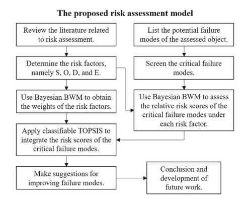
统计代写|决策与风险作业代写decision and risk代考|The Proposed Risk Assessment Model
如果你也在 怎样代写决策与风险decision and risk这个学科遇到相关的难题,请随时右上角联系我们的24/7代写客服。
决策与风险分析帮助组织在存在风险和不确定性的情况下做出决策,使其效用最大化。
风险决策。一个组织的领导层决定接受一个具有特定风险功能的选项,而不是另一个,或者是不采取任何行动。我认为,任何有价值的组织的主管领导都可以在适当的级别上做出这样的决定。
这个术语是在备选方案之间做出决定的简称,其中至少有一个方案有损失的概率。(通常在网络风险中,我们关注的是损失,但所有的想法都自然地延伸到上升或机会风险。很少有人和更少的组织会在没有预期利益的情况下承担风险,即使只是避免成本)。
损失大小的概率分布,在某个规定的时间段,如一年。这就是我认为大多数人在谈论某物的 “风险 “时的真正含义。
statistics-lab™ 为您的留学生涯保驾护航 在代写决策与风险decision and risk方面已经树立了自己的口碑, 保证靠谱, 高质且原创的统计Statistics代写服务。我们的专家在代写决策与风险decision and risk方面经验极为丰富,各种代写决策与风险decision and risk相关的作业也就用不着说。
我们提供的决策与风险decision and risk及其相关学科的代写,服务范围广, 其中包括但不限于:
- Statistical Inference 统计推断
- Statistical Computing 统计计算
- Advanced Probability Theory 高等楖率论
- Advanced Mathematical Statistics 高等数理统计学
- (Generalized) Linear Models 广义线性模型
- Statistical Machine Learning 统计机器学习
- Longitudinal Data Analysis 纵向数据分析
- Foundations of Data Science 数据科学基础
统计代写|决策与风险作业代写decision and risk代考|Bayesian BWM
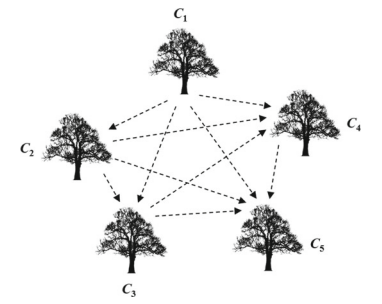
In order to more objective integrate the opinions of multiple risk analysts, Mohammadi and Rezaei $(2020)$ developed a probabilistic model of BWM, called Bayesian BWM. Because the judgments provided by each decision-maker in BWM are different, the two vectors information would be different (risk analysts may choose
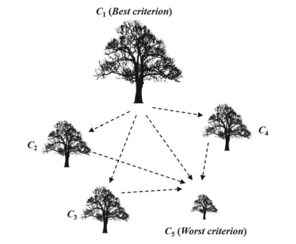
different best/worst evaluated item). Therefore, it is not possible to aggregate the opinions of multiple risk analysts by using arithmetic averages. The weight vector of the MCDM is $w_{j}=\left(w_{1}, w_{2}, \ldots, w_{j}, \ldots, w_{n}\right)$, with $\sum_{j=1}^{n} w_{j}=1$ and $w_{j} \geq 0$ required. Each $w_{j}$ is represented as the weight of the corresponding evaluated item $C_{j}$. The evaluated item $C_{j}$ can be regarded as a random event, and the weight $w_{j}$ is their occurrence probability. According to probability theory, the same is true for $\sum_{j=1}^{n} w_{j}=1$ and $w_{j} \geq 0$. Therefore, it is feasible to construct a probability model from the perspective of decision-making. The execution steps are as follows (Mohammadi and Rezaei 2020):
Steps 1-4. The same as Steps $1-4$ of conventional BWM.
Step 5. Calculate the best weight value of the group of evaluated items.
The input data $A_{B}$ and $A_{W}$ of the BWM can be builded as a probability model of polynomial distribution. The contents of the two vectors are both positive integers, the probability mass function of the polynomial distribution of a given $A_{W}$ is
$$
P\left(A_{W} \mid w\right)=\frac{\left(\sum_{j=1}^{n} a_{j w}\right) !}{\prod_{j=1}^{n} a_{j w} !} \prod_{j=1}^{n} w_{j}^{a_{j w}}
$$
where $w$ is the polynomial distribution, the probability of event $j$ is proportional to the number of occurrences and the total number of experiments.
$$
w_{j} \propto \frac{a_{j w}}{\sum_{j=1}^{n} a_{j w}}, \forall j=1,2, \ldots, n .
$$
Similarly, the worst evaluated item $C_{W}$ can be written as follows:
$$
w_{W} \propto \frac{a_{W W}}{\sum_{j=1}^{n} a_{j W}}=\frac{1}{\sum_{j=1}^{n} a_{j W}} .
$$
Equations (2.6) and (2.7) can be integrated to obtain the following:
$$
\frac{w_{j}}{w_{W}} \propto a_{j w}, \forall j=1,2, \ldots, n
$$
Besides, $A_{B}$ is modeled using polynomial distribution. However, the concepts of the generation of $A_{B}$ and $A_{W}$ are different. The former is the optimal evaluated item $B$ compared to the other evaluated items $j$. The larger the evaluation value, the smaller the weight of the compared evaluated item $j$; the latter refers to other evaluated items. The evaluation item $j$ is compared with the worst evaluated item $W$. The larger the evaluation value, the greater the weight of the evaluated item $j$. Therefore, the conversion of the assessment content of $A_{B}$ into the weight should be reciprocal.
统计代写|决策与风险作业代写decision and risk代考|Classifiable TOPSIS Technique
TOPSIS technique is one of the most popular sorting methods for ranking the evaluated items. This method is to determine the relative position of each evaluated item by determining the degree of separation between each evaluated item and the positive and negative ideal solutions (PIS and NIS). The optimal evaluated item is the one closest to the PIS and the farthest away from the NIS. In risk management, the
closer to the positive ideal solution, the greater the degree of risk. TOPSIS will not affect the time and quality of the solution due to the number of evaluated items. In addition, this paper applies classifiable TOPSIS technique (Liaw et al. 2020), which can not only obtain a more reliable ranking, but also divide all the evaluated items into four risk levels. When a new evaluated item is added, the method can be used to immediately assign a level to it. The detailed classifiable TOPSIS technique steps are described as follows (Liaw et al. 2020):
Step 1. Build the initial evaluation matrix $\boldsymbol{X}$
Assume that there are $i$ evaluated items in the risk assessment framework, $i=1$, $2, \ldots, m ; j$ represents 4 risk factors, $\mathrm{S}, \mathrm{O}, \mathrm{D}$, and $\mathrm{E}$. Under each risk factor, the risk values of the evaluated items are evaluated to obtain the initial evaluation matrix. In the paper, Bayesian BWM is used to obtain the content of the matrix.
$$
\mathcal{X}=\left[\begin{array}{cccc}
d_{1 S} & d_{1 O} & d_{1 D} & d_{1 E} \
d_{2 S} & d_{2 O} & d_{2 D} & d_{2 E} \
\vdots & \vdots & \vdots & \vdots \
d_{i S} & d_{i O} & d_{i D} & d_{i E} \
\vdots & \vdots & \vdots & \vdots \
d_{m S} & d_{m O} & d_{m D} & d_{m E}
\end{array}\right], i=1,2,
$$
Step 2. Calculate the normalized evaluation matrix $X^{*}$
Because the data range obtained through Bayesian BWM is already between 0 and 1. Therefore, this step does not need to be executed.
统计代写|决策与风险作业代写decision and risk代考|Problem Description
The practicality and effectiveness of the developed risk assessment model can be illustrated through a practical case. The reliability and robustness of machine tools are very important to the manufacturing industry, because it is the main production equipment in the manufacturing industry. Quality control engineers or risk analysts must implement risk assessment and improvement plans for new products to reduce the occurrence of product failures. The company in this case is a multinational manufacturer of machine tool parts in Taiwan. The company’s machine tool components include computer numerical control (CNC) rotary tables, indexing tables, hydraulic indexing tables, auto-pallet changer with worktable, etc. In the face of a competitive global market, the company must develop products that are more stable, more precise, faster, and more functional. Therefore, the company implements FMEA activities before the launch of various new products.
The FMEA team was composed of senior department heads of the company. There were seven risk analysts from six different departments, including business department, design department, manufacturing department, quality control department, management department, and sales service department. The seven risk analysts had more than 15 years of experience in the machine tool manufacturing industry and have participated in machine tool related international exhibitions for many times. In addition to their professional technical knowledge, they also understood the development trend of machine tools. In the study, the case company used a newly developed computer numerical control (CNC) rotary table as the product of FMEA analysis, which is CNC rotary tilting Table 250 (TRT-250). As an NC controlled 2 axis table, TRT-250 is suitable for larger workloads in 5 axis machining. A one-piece housing structure with a powerful hydraulic clamping system offers a greater clamping torque and high loading capacities. It is also designed for easy installation and alignment. The FMEA team listed all the failure modes and evaluated the key failure modes, as shown in Table 2.7.
It can be seen from Table $2.7$ that there are nine critical failure modes. They are the rotating shaft segmentation accuracy exceeding the standard (FM1), the rotating shaft reproducibility exceeding the standard (FM2), the positive/negative clearance of the rotating shaft exceeding the standard (FM3), the inclined shaft reproducibility exceeding the standard (FM4), the positive/negative clearance of the inclined shaft exceeding the standard (FM5), the machine making noise when the inclined shaft rotates (FM6), abnormal proximity switch (FM7), oil leakage from the disk surface (FM8), and improper waterproof measures (FM9). FMEA was performed to further analyze them.
决策与风险代写
统计代写|决策与风险作业代写decision and risk代考|Bayesian BWM
为了更客观地整合多位风险分析师 Mohammadi 和 Rezaei 的意见(2020)开发了 BWM 的概率模型,称为贝叶斯 BWM。由于 BWM 中每个决策者提供的判断不同,因此两个向量信息会不同(风险分析师可能会选择
不同的最佳/最差评估项目)。因此,不可能使用算术平均来汇总多个风险分析师的意见。MCDM 的权重向量为在j=(在1,在2,…,在j,…,在n), 和∑j=1n在j=1和在j≥0必需的。每个在j表示为对应评估项的权重Cj. 评估项目Cj可以看作是一个随机事件,权重在j是它们的发生概率。根据概率论,同样适用于∑j=1n在j=1和在j≥0. 因此,从决策的角度构建概率模型是可行的。执行步骤如下(Mohammadi and Rezaei 2020):
步骤 1-4。与步骤相同1−4常规 BWM。
Step 5. 计算评估项目组的最佳权重值。
输入数据一种乙和一种在BWM 可以构建为多项式分布的概率模型。两个向量的内容都是正整数,给定多项式分布的概率质量函数一种在是
磷(一种在∣在)=(∑j=1n一种j在)!∏j=1n一种j在!∏j=1n在j一种j在
在哪里在是多项式分布,事件的概率j与出现次数和实验总数成正比。
在j∝一种j在∑j=1n一种j在,∀j=1,2,…,n.
同样,评估最差的项目C在可以写成如下:
在在∝一种在在∑j=1n一种j在=1∑j=1n一种j在.
等式 (2.6) 和 (2.7) 可以积分得到以下结果:
在j在在∝一种j在,∀j=1,2,…,n
除了,一种乙使用多项式分布建模。但是,生成的概念一种乙和一种在是不同的。前者为最优评价项目乙与其他评估项目相比j. 评价值越大,被比较评价项目的权重越小j; 后者指其他评估项目。评价项目j与评估最差的项目进行比较在. 评价值越大,评价项目的权重越大j. 因此,评估内容的转换一种乙进的重量应该是倒数。
统计代写|决策与风险作业代写decision and risk代考|Classifiable TOPSIS Technique
TOPSIS技术是最流行的排序方法之一,用于对评估项目进行排名。该方法是通过确定每个被评估项目与正负理想解(PIS和NIS)之间的分离程度来确定每个被评估项目的相对位置。最优评价项目是最接近 PIS 和最远离 NIS 的项目。在风险管理中,
越接近正理想解,风险程度越大。TOPSIS 不会因为评估项目的数量而影响解决方案的时间和质量。此外,本文应用了可分类TOPSIS技术(Liaw et al. 2020),不仅可以获得更可靠的排名,而且将所有评估项目分为四个风险等级。当添加一个新的评估项目时,该方法可用于立即为其分配一个级别。详细的可分类 TOPSIS 技术步骤描述如下(Liaw et al. 2020):
步骤 1. 建立初始评估矩阵X
假设有一世风险评估框架中的评估项目,一世=1,2,…,米;j代表4个风险因素,小号,这,D, 和和. 在每个风险因素下,对被评估项目的风险值进行评估,得到初始评估矩阵。论文中使用贝叶斯BWM来获取矩阵的内容。
X=[d1小号d1这d1Dd1和 d2小号d2这d2Dd2和 ⋮⋮⋮⋮ d一世小号d一世这d一世Dd一世和 ⋮⋮⋮⋮ d米小号d米这d米Dd米和],一世=1,2,
步骤 2. 计算归一化评估矩阵X∗
因为通过贝叶斯BWM得到的数据范围已经在0到1之间,所以不需要执行这一步。
统计代写|决策与风险作业代写decision and risk代考|Problem Description
所开发的风险评估模型的实用性和有效性可以通过一个实际案例来说明。机床的可靠性和坚固性对制造业来说非常重要,因为它是制造业的主要生产设备。质量控制工程师或风险分析师必须对新产品实施风险评估和改进计划,以减少产品故障的发生。本案中的公司是台湾一家跨国机床零件制造商。公司的机床部件包括计算机数控(CNC)转台、分度台、液压分度台、带工作台的自动托盘交换装置等。面对竞争激烈的全球市场,公司必须开发更稳定、更稳定的产品,更精确,更快,并且更实用。因此,公司在推出各种新产品之前就实施了FMEA活动。
FMEA团队由公司高级部门负责人组成。风险分析师7人,分别来自业务部、设计部、制造部、品管部、管理部、销售服务部六个部门。七位风险分析师在机床制造行业拥有超过15年的经验,并多次参加机床相关的国际展会。除了专业的技术知识外,他们还了解机床的发展趋势。在研究中,案例公司使用了新开发的计算机数控(CNC)转台作为FMEA分析的产品,即CNC转台250(TRT-250)。作为 NC 控制的 2 轴工作台,TRT-250 适用于 5 轴加工中较大的工作量。具有强大液压夹紧系统的一体式外壳结构提供更大的夹紧扭矩和高负载能力。它还设计为易于安装和对齐。FMEA 团队列出了所有失效模式并评估了关键失效模式,如表 2.7 所示。
从表中可以看出2.7有九种关键故障模式。分别是转轴分段精度超标(FM1)、转轴再现性超标(FM2)、转轴正负游隙超标(FM3)、斜轴再现性超标(FM4) )、斜轴正负游隙超标(FM5)、斜轴转动时机器发出异响(FM6)、接近开关异常(FM7)、盘面漏油(FM8)、不当防水措施 (FM9)。进行 FMEA 以进一步分析它们。

统计代写请认准statistics-lab™. statistics-lab™为您的留学生涯保驾护航。统计代写|python代写代考
随机过程代考
在概率论概念中,随机过程是随机变量的集合。 若一随机系统的样本点是随机函数,则称此函数为样本函数,这一随机系统全部样本函数的集合是一个随机过程。 实际应用中,样本函数的一般定义在时间域或者空间域。 随机过程的实例如股票和汇率的波动、语音信号、视频信号、体温的变化,随机运动如布朗运动、随机徘徊等等。
贝叶斯方法代考
贝叶斯统计概念及数据分析表示使用概率陈述回答有关未知参数的研究问题以及统计范式。后验分布包括关于参数的先验分布,和基于观测数据提供关于参数的信息似然模型。根据选择的先验分布和似然模型,后验分布可以解析或近似,例如,马尔科夫链蒙特卡罗 (MCMC) 方法之一。贝叶斯统计概念及数据分析使用后验分布来形成模型参数的各种摘要,包括点估计,如后验平均值、中位数、百分位数和称为可信区间的区间估计。此外,所有关于模型参数的统计检验都可以表示为基于估计后验分布的概率报表。
广义线性模型代考
广义线性模型(GLM)归属统计学领域,是一种应用灵活的线性回归模型。该模型允许因变量的偏差分布有除了正态分布之外的其它分布。
statistics-lab作为专业的留学生服务机构,多年来已为美国、英国、加拿大、澳洲等留学热门地的学生提供专业的学术服务,包括但不限于Essay代写,Assignment代写,Dissertation代写,Report代写,小组作业代写,Proposal代写,Paper代写,Presentation代写,计算机作业代写,论文修改和润色,网课代做,exam代考等等。写作范围涵盖高中,本科,研究生等海外留学全阶段,辐射金融,经济学,会计学,审计学,管理学等全球99%专业科目。写作团队既有专业英语母语作者,也有海外名校硕博留学生,每位写作老师都拥有过硬的语言能力,专业的学科背景和学术写作经验。我们承诺100%原创,100%专业,100%准时,100%满意。
机器学习代写
随着AI的大潮到来,Machine Learning逐渐成为一个新的学习热点。同时与传统CS相比,Machine Learning在其他领域也有着广泛的应用,因此这门学科成为不仅折磨CS专业同学的“小恶魔”,也是折磨生物、化学、统计等其他学科留学生的“大魔王”。学习Machine learning的一大绊脚石在于使用语言众多,跨学科范围广,所以学习起来尤其困难。但是不管你在学习Machine Learning时遇到任何难题,StudyGate专业导师团队都能为你轻松解决。
多元统计分析代考
基础数据: $N$ 个样本, $P$ 个变量数的单样本,组成的横列的数据表
变量定性: 分类和顺序;变量定量:数值
数学公式的角度分为: 因变量与自变量
时间序列分析代写
随机过程,是依赖于参数的一组随机变量的全体,参数通常是时间。 随机变量是随机现象的数量表现,其时间序列是一组按照时间发生先后顺序进行排列的数据点序列。通常一组时间序列的时间间隔为一恒定值(如1秒,5分钟,12小时,7天,1年),因此时间序列可以作为离散时间数据进行分析处理。研究时间序列数据的意义在于现实中,往往需要研究某个事物其随时间发展变化的规律。这就需要通过研究该事物过去发展的历史记录,以得到其自身发展的规律。
回归分析代写
多元回归分析渐进(Multiple Regression Analysis Asymptotics)属于计量经济学领域,主要是一种数学上的统计分析方法,可以分析复杂情况下各影响因素的数学关系,在自然科学、社会和经济学等多个领域内应用广泛。
MATLAB代写
MATLAB 是一种用于技术计算的高性能语言。它将计算、可视化和编程集成在一个易于使用的环境中,其中问题和解决方案以熟悉的数学符号表示。典型用途包括:数学和计算算法开发建模、仿真和原型制作数据分析、探索和可视化科学和工程图形应用程序开发,包括图形用户界面构建MATLAB 是一个交互式系统,其基本数据元素是一个不需要维度的数组。这使您可以解决许多技术计算问题,尤其是那些具有矩阵和向量公式的问题,而只需用 C 或 Fortran 等标量非交互式语言编写程序所需的时间的一小部分。MATLAB 名称代表矩阵实验室。MATLAB 最初的编写目的是提供对由 LINPACK 和 EISPACK 项目开发的矩阵软件的轻松访问,这两个项目共同代表了矩阵计算软件的最新技术。MATLAB 经过多年的发展,得到了许多用户的投入。在大学环境中,它是数学、工程和科学入门和高级课程的标准教学工具。在工业领域,MATLAB 是高效研究、开发和分析的首选工具。MATLAB 具有一系列称为工具箱的特定于应用程序的解决方案。对于大多数 MATLAB 用户来说非常重要,工具箱允许您学习和应用专业技术。工具箱是 MATLAB 函数(M 文件)的综合集合,可扩展 MATLAB 环境以解决特定类别的问题。可用工具箱的领域包括信号处理、控制系统、神经网络、模糊逻辑、小波、仿真等。