如果你也在 怎样代写傅立叶光学Fourier optics这个学科遇到相关的难题，请随时右上角联系我们的24/7代写客服。

傅里叶光学是利用傅里叶变换（FTs）对经典光学的研究，其中所考虑的波形被认为是由平面波的组合或叠加组成的。

statistics-lab™ 为您的留学生涯保驾护航 在代写傅立叶光学Fourier optics方面已经树立了自己的口碑, 保证靠谱, 高质且原创的统计Statistics代写服务。我们的专家在代写傅立叶光学Fourier optics代写方面经验极为丰富，各种代写傅立叶光学Fourier optics相关的作业也就用不着说。

我们提供的傅立叶光学Fourier optics及其相关学科的代写，服务范围广, 其中包括但不限于:

• Statistical Inference 统计推断
• Statistical Computing 统计计算
• Advanced Probability Theory 高等概率论
• Advanced Mathematical Statistics 高等数理统计学
• (Generalized) Linear Models 广义线性模型
• Statistical Machine Learning 统计机器学习
• Longitudinal Data Analysis 纵向数据分析
• Foundations of Data Science 数据科学基础

物理代写|傅立叶光学代写Fourier optics代考|Sampling by averaging, distributions

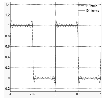
We will now learn the important idea of the delta function that will be handy later in this book. Sampling a continuous function is a part of every measurement or digitization process. Suppose we have a signal $I(x)$ – say the intensity of ambient light along a line on a screen – that we wish to sample at discrete set of points $x_1, x_2, \ldots$. How do we go about it? Every detector we can possibly use to measure the intensity will have some finite width $2 L$ and a sample of $I(x)$ will be an average over this detector area. So we may write the intensity at point $x=0$, or $I(0)$ as:
$$
I(0) \approx \frac{1}{2 L} \int_{-\infty}^{\infty} d x I(x) \operatorname{rect}\left(\frac{x}{2 L}\right) .
$$
Now how do we improve this approximation so that we go to the ideal $I(0)$ ? Clearly we have to reduce the size $2 L$ over which the average is carried out. We may say that:
$$
I(0)=\lim {2 L \rightarrow 0} \frac{1}{2 L} \int{-\infty}^{\infty} d x I(x) \operatorname{rect}\left(\frac{x}{2 L}\right) .
$$
Notice that as the length $2 L \rightarrow 0$ the width of the function $\frac{1}{2 L} \operatorname{rect}\left(\frac{x}{2 L}\right)$ keeps reducing whereas its height keeps increasing such that the area under the curve is unity. This limiting process leads us to an impulse which is also commonly known by the name delta function. We may write:
$$
\delta(x)=\lim _{2 L \rightarrow 0} \frac{1}{2 L} \operatorname{rect}\left(\frac{x}{2 L}\right) .
$$
Although it is commonly referred to as the “delta function” and we will often call it that way, you will appreciate that it is not a function in the usual sense. When we say $f(x)=x^2$ we are associating a value for every input number $x$. The impulse or delta distribution is more of an idea that is the result of a limiting process. Anything that is equal to zero everywhere in the limit except at $x=0$, where it tends to infinity cannot be a function in the sense you may have learnt in your mathematics classes.

物理代写|傅立叶光学代写Fourier optics代考|Properties of delta function

1. Sampling property At points of continuity of a function $g(x)$ we have:
   $$
   \int_{-\infty}^{\infty} d x g(x) \delta\left(x \quad x^{\prime}\right)=g\left(x^{\prime}\right) .
   $$
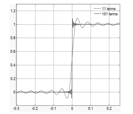
   If at $x=x^{\prime}$ the function $g(x)$ has a finite jump discontinuity, the right hand side of the above equation is an average value of the two limits $g\left(x_{+}^{\prime}\right)$ and $g\left(x_{-}^{\prime}\right)$.
2. Derivatives of delta function All operations with delta function are to be associated with a test function under integral sign. We evaluate the integral below by parts.
   $$
   \begin{aligned}
   \int_{-\infty}^{\infty} & d x g(x) \frac{d}{d x} \delta\left(x-x^{\prime}\right) \
   &=\left.g(x) \delta\left(x-x^{\prime}\right)\right|{-\infty} ^{\infty}-\int{-\infty}^{\infty} d x \frac{d}{d x} g(x) \delta\left(x-x^{\prime}\right) \
   &=-g^{\prime}\left(x^{\prime}\right) .
   \end{aligned}
   $$
   This property applies to multiple order derivatives. So continuing along the lines of above equation we get:
   $$
   \int_{-\infty}^{\infty} d x g(x) \frac{d^n}{d x^n} \delta\left(x-x^{\prime}\right)=(-1)^n g^{(n)}\left(x^{\prime}\right),
   $$
   where $g^{(n)}(x)$ is the $\mathrm{n}$-th order derivative of $g(x)$.
3. Delta function with scaling First of all we note that the delta function is even: $\delta(-x)=\delta(x)$. This leads to:
   $$
   \begin{aligned}
   \int_{-\infty}^{\infty} d x g(x) \delta(a x) &=\frac{1}{|a|} \int_{-\infty}^{\infty} d x g\left(\frac{x}{a}\right) \delta(x) \
   &=\frac{1}{|a|} g(0)
   \end{aligned}
   $$
   We may therefore write: $\delta(a x)=\frac{1}{|a|} \delta(x)$.

傅立叶光学代考

物理代写|傅立叶光学代写傅里叶光学代考|通过平均采样，分布

我们现在将学习增量函数的重要思想，这将在本书后面很方便。对连续函数采样是每一个测量或数字化过程的一部分。假设我们有一个信号$I(x)$——比如屏幕上一条直线上的环境光的强度——我们希望在$x_1, x_2, \ldots$的离散点集合上对其进行采样。我们该怎么做呢?我们可能用来测量强度的每个探测器都有一个有限的宽度$2 L$, $I(x)$的样本将是这个探测器区域的平均值。所以我们可以把点$x=0$或$I(0)$的强度写成:
$$
I(0) \approx \frac{1}{2 L} \int_{-\infty}^{\infty} d x I(x) \operatorname{rect}\left(\frac{x}{2 L}\right) .
$$
现在我们如何改进这个近似，使我们达到理想的$I(0)$ ?很明显，我们必须减少$2 L$的规模，在这个规模上进行平均数。我们可以说:
$$
I(0)=\lim {2 L \rightarrow 0} \frac{1}{2 L} \int{-\infty}^{\infty} d x I(x) \operatorname{rect}\left(\frac{x}{2 L}\right) .
$$
请注意，随着长度$2 L \rightarrow 0$，函数$\frac{1}{2 L} \operatorname{rect}\left(\frac{x}{2 L}\right)$的宽度不断减少，而它的高度不断增加，因此曲线下的面积是单位的。这个极限过程使我们得到一个脉冲，它通常被称为脉冲函数。我们可以这样写:
$$
\delta(x)=\lim _{2 L \rightarrow 0} \frac{1}{2 L} \operatorname{rect}\left(\frac{x}{2 L}\right) .
$$
尽管它通常被称为“增量函数”，我们也经常这样称呼它，但你会意识到它不是通常意义上的函数。当我们说$f(x)=x^2$时，我们是在为每个输入数字$x$关联一个值。脉冲分布更像是极限过程的结果。任何在极限处都等于零的东西，除了在$x=0$处，它趋于无穷，不可能是你在数学课上学到的那种意义上的函数。

物理代写|傅立叶光学代写傅里叶光学代考|函数的性质

1. 采样性质在函数的连续性点上 $g(x)$ 我们有:
   $$
   \int_{-\infty}^{\infty} d x g(x) \delta\left(x \quad x^{\prime}\right)=g\left(x^{\prime}\right) .
   $$
   如果at $x=x^{\prime}$ 函数 $g(x)$ 有一个有限跳跃不连续，上面方程的右边是两个极限的平均值 $g\left(x_{+}^{\prime}\right)$ 和 $g\left(x_{-}^{\prime}\right)$
2. δ函数的导数所有关于δ函数的运算都与积分符号下的测试函数相关联。我们用分部计算下面的积分。
   $$
   \begin{aligned}
   \int_{-\infty}^{\infty} & d x g(x) \frac{d}{d x} \delta\left(x-x^{\prime}\right) \
   &=\left.g(x) \delta\left(x-x^{\prime}\right)\right|{-\infty} ^{\infty}-\int{-\infty}^{\infty} d x \frac{d}{d x} g(x) \delta\left(x-x^{\prime}\right) \
   &=-g^{\prime}\left(x^{\prime}\right) .
   \end{aligned}
   $$
   此属性适用于多个阶导数。所以继续沿着上面的等式，我们得到:
   $$
   \int_{-\infty}^{\infty} d x g(x) \frac{d^n}{d x^n} \delta\left(x-x^{\prime}\right)=(-1)^n g^{(n)}\left(x^{\prime}\right),
   $$
   where $g^{(n)}(x)$ 是 $\mathrm{n}$的-阶导数 $g(x)$.
3. 带缩放的函数首先我们注意到函数是偶的: $\delta(-x)=\delta(x)$。这将导致:
   $$
   \begin{aligned}
   \int_{-\infty}^{\infty} d x g(x) \delta(a x) &=\frac{1}{|a|} \int_{-\infty}^{\infty} d x g\left(\frac{x}{a}\right) \delta(x) \
   &=\frac{1}{|a|} g(0)
   \end{aligned}
   $$因此，我们可以这样写: $\delta(a x)=\frac{1}{|a|} \delta(x)$.

统计代写请认准statistics-lab™. statistics-lab™为您的留学生涯保驾护航。

金融工程代写

金融工程是使用数学技术来解决金融问题。金融工程使用计算机科学、统计学、经济学和应用数学领域的工具和知识来解决当前的金融问题，以及设计新的和创新的金融产品。

非参数统计代写

非参数统计指的是一种统计方法，其中不假设数据来自于由少数参数决定的规定模型；这种模型的例子包括正态分布模型和线性回归模型。

广义线性模型代考

广义线性模型（GLM）归属统计学领域，是一种应用灵活的线性回归模型。该模型允许因变量的偏差分布有除了正态分布之外的其它分布。

术语 广义线性模型（GLM）通常是指给定连续和/或分类预测因素的连续响应变量的常规线性回归模型。它包括多元线性回归，以及方差分析和方差分析（仅含固定效应）。

有限元方法代写

有限元方法（FEM）是一种流行的方法，用于数值解决工程和数学建模中出现的微分方程。典型的问题领域包括结构分析、传热、流体流动、质量运输和电磁势等传统领域。

有限元是一种通用的数值方法，用于解决两个或三个空间变量的偏微分方程（即一些边界值问题）。为了解决一个问题，有限元将一个大系统细分为更小、更简单的部分，称为有限元。这是通过在空间维度上的特定空间离散化来实现的，它是通过构建对象的网格来实现的：用于求解的数值域，它有有限数量的点。边界值问题的有限元方法表述最终导致一个代数方程组。该方法在域上对未知函数进行逼近。[1] 然后将模拟这些有限元的简单方程组合成一个更大的方程系统，以模拟整个问题。然后，有限元通过变化微积分使相关的误差函数最小化来逼近一个解决方案。

tatistics-lab作为专业的留学生服务机构，多年来已为美国、英国、加拿大、澳洲等留学热门地的学生提供专业的学术服务，包括但不限于Essay代写，Assignment代写，Dissertation代写，Report代写，小组作业代写，Proposal代写，Paper代写，Presentation代写，计算机作业代写，论文修改和润色，网课代做，exam代考等等。写作范围涵盖高中，本科，研究生等海外留学全阶段，辐射金融，经济学，会计学，审计学，管理学等全球99%专业科目。写作团队既有专业英语母语作者，也有海外名校硕博留学生，每位写作老师都拥有过硬的语言能力，专业的学科背景和学术写作经验。我们承诺100%原创，100%专业，100%准时，100%满意。

随机分析代写

随机微积分是数学的一个分支，对随机过程进行操作。它允许为随机过程的积分定义一个关于随机过程的一致的积分理论。这个领域是由日本数学家伊藤清在第二次世界大战期间创建并开始的。

时间序列分析代写

随机过程，是依赖于参数的一组随机变量的全体，参数通常是时间。 随机变量是随机现象的数量表现，其时间序列是一组按照时间发生先后顺序进行排列的数据点序列。通常一组时间序列的时间间隔为一恒定值（如1秒，5分钟，12小时，7天，1年），因此时间序列可以作为离散时间数据进行分析处理。研究时间序列数据的意义在于现实中，往往需要研究某个事物其随时间发展变化的规律。这就需要通过研究该事物过去发展的历史记录，以得到其自身发展的规律。

回归分析代写

多元回归分析渐进（Multiple Regression Analysis Asymptotics）属于计量经济学领域，主要是一种数学上的统计分析方法，可以分析复杂情况下各影响因素的数学关系，在自然科学、社会和经济学等多个领域内应用广泛。

MATLAB代写

MATLAB 是一种用于技术计算的高性能语言。它将计算、可视化和编程集成在一个易于使用的环境中，其中问题和解决方案以熟悉的数学符号表示。典型用途包括：数学和计算算法开发建模、仿真和原型制作数据分析、探索和可视化科学和工程图形应用程序开发，包括图形用户界面构建MATLAB 是一个交互式系统，其基本数据元素是一个不需要维度的数组。这使您可以解决许多技术计算问题，尤其是那些具有矩阵和向量公式的问题，而只需用 C 或 Fortran 等标量非交互式语言编写程序所需的时间的一小部分。MATLAB 名称代表矩阵实验室。MATLAB 最初的编写目的是提供对由 LINPACK 和 EISPACK 项目开发的矩阵软件的轻松访问，这两个项目共同代表了矩阵计算软件的最新技术。MATLAB 经过多年的发展，得到了许多用户的投入。在大学环境中，它是数学、工程和科学入门和高级课程的标准教学工具。在工业领域，MATLAB 是高效研究、开发和分析的首选工具。MATLAB 具有一系列称为工具箱的特定于应用程序的解决方案。对于大多数 MATLAB 用户来说非常重要，工具箱允许您学习和应用专业技术。工具箱是 MATLAB 函数（M 文件）的综合集合，可扩展 MATLAB 环境以解决特定类别的问题。可用工具箱的领域包括信号处理、控制系统、神经网络、模糊逻辑、小波、仿真等。

R语言代写	问卷设计与分析代写
PYTHON代写	回归分析与线性模型代写
MATLAB代写	方差分析与试验设计代写
STATA代写	机器学习/统计学习代写
SPSS代写	计量经济学代写
EVIEWS代写	时间序列分析代写
EXCEL代写	深度学习代写
SQL代写	各种数据建模与可视化代写

如果你也在 怎样代写傅立叶光学Fourier optics这个学科遇到相关的难题，请随时右上角联系我们的24/7代写客服。

傅里叶光学是利用傅里叶变换（FTs）对经典光学的研究，其中所考虑的波形被认为是由平面波的组合或叠加组成的。

statistics-lab™ 为您的留学生涯保驾护航 在代写傅立叶光学Fourier optics方面已经树立了自己的口碑, 保证靠谱, 高质且原创的统计Statistics代写服务。我们的专家在代写傅立叶光学Fourier optics代写方面经验极为丰富，各种代写傅立叶光学Fourier optics相关的作业也就用不着说。

我们提供的傅立叶光学Fourier optics及其相关学科的代写，服务范围广, 其中包括但不限于:

• Statistical Inference 统计推断
• Statistical Computing 统计计算
• Advanced Probability Theory 高等概率论
• Advanced Mathematical Statistics 高等数理统计学
• (Generalized) Linear Models 广义线性模型
• Statistical Machine Learning 统计机器学习
• Longitudinal Data Analysis 纵向数据分析
• Foundations of Data Science 数据科学基础

物理代写|傅立叶光学代写Fourier optics代考|Fourier transform as a limiting case of Fourier series

We will now consider the limiting case of the Fourier series as the period $T$ goes to $\infty$. It is clear that the function $g(x)$ is no more periodic. We denote the discrete frequencies as:
$$
f_{x n}=\frac{n}{T},
$$
The difference between the consecutive discrete frequencies is given by $\Delta f_x=f_{x(n+1)}-f_{x n}=1 / T$. Further we define:
$$
G\left(f_{x n}\right)=\int_{-\infty}^{\infty} d x g(x) \exp \left(-i 2 \pi f_{x n} x\right) .
$$
We may write the Fourier series expansion as:
$$
\begin{aligned}
g(x) &=\sum_{n=-\infty}^{\infty} G_n \exp \left(i 2 \pi f_{x n} x\right) \
&=\sum_{n=-\infty}^{\infty}\left[\frac{1}{T} \int_{-T / 2}^{T / 2} d x^{\prime} g\left(x^{\prime}\right) \exp \left(-i 2 \pi f_{x n} x^{\prime}\right)\right] \exp \left(i 2 \pi f_{x n} x\right) .
\end{aligned}
$$
In the limit $T \rightarrow \infty$ we have:
$$
\begin{aligned}
g(x) & \rightarrow \sum_{n=-\infty}^{\infty} G\left(f_{x n}\right) \exp \left(i 2 \pi f_{x n} x\right) \Delta f_x \
& \rightarrow \int_{-\infty}^{\infty} d f_x G\left(f_x\right) \exp \left(i 2 \pi f_x x\right)
\end{aligned}
$$

物理代写|傅立叶光学代写Fourier optics代考|Fourier transform of the rectangle distribution

The Fourier transform of the rect function may be evaluated as:
$$
\begin{aligned}
G\left(f_x\right) &=\int_{-L}^L d x \exp \left(-i 2 \pi f_x x\right) \
&=\left[\frac{\exp \left(-i 2 \pi f_x x\right)}{-i 2 \pi f_x}\right]{-L}^L \ &=2 L \frac{\sin \left(2 \pi f_x L\right)}{\left(2 \pi f_x L\right)} \ &=2 L \operatorname{sinc}\left(2 L f_x\right) \end{aligned} $$ Here the sinc-function is as defined in Eq. (2.21). Note that although $\operatorname{rect}(x)$ has a discontinuity, its transform is continuous. Further it is somewhat surprising to know that $\left|\operatorname{sinc}\left(f_x\right)\right|$ is not absolutely integrable to have a Fourier transform or Fourier inverse in the conventional sense required by the Dirichlet sufficiency conditions. To show this consider the intervals along $f_x$ axis where $\left|\sin \left(\pi f_x\right)\right| \geq$ $0.5$. These intervals are given by $f_x \in[n+1 / 6, n+5 / 6]$. We therefore have: $$ \int{-\infty}^{\infty} d f_x\left|\operatorname{sinc}\left(f_x\right)\right|>2 \frac{1}{2 \pi} \sum_{n=0}^{\infty} \frac{2 / 3}{n+5 / 6} \rightarrow \infty
$$
The series on the right hand side diverges and as a result the absolute integral of $\operatorname{sinc}\left(f_x\right)$ does not exist. Functions such as spikes, steps and even ever extending sines and cosines do not have a Fourier transform in traditional theory. Defining Fourier transforms for such functions is however a practical necessity when representing images as $2 \mathrm{D}$ matrices in digital form. In fact edges or spikes contain most important visual information in images. The traditional Fourier transform theory must therefore be extended to take these cases into account. We will study the important case of the Dirac delta function in this context. This class of functions (spikes, steps, etc) with no Fourier transform in conventional theory is known by the name generalized functions. We will not deal with theory of generalized functions in detail but study some specific cases of interest starting with the Dirac delta function.

傅立叶光学代考

物理代写|傅立叶光学代写傅立叶光学代考|傅立叶变换作为傅立叶级数的极限情况

我们现在考虑傅里叶级数的极限情况，当周期$T$到$\infty$。很明显，函数$g(x)$不再具有周期性。我们将离散频率表示为:
$$
f_{x n}=\frac{n}{T},
$$
连续离散频率之间的差由$\Delta f_x=f_{x(n+1)}-f_{x n}=1 / T$给出。我们进一步定义:
$$
G\left(f_{x n}\right)=\int_{-\infty}^{\infty} d x g(x) \exp \left(-i 2 \pi f_{x n} x\right) .
$$
我们可以把傅里叶级数展开写成:
$$
\begin{aligned}
g(x) &=\sum_{n=-\infty}^{\infty} G_n \exp \left(i 2 \pi f_{x n} x\right) \
&=\sum_{n=-\infty}^{\infty}\left[\frac{1}{T} \int_{-T / 2}^{T / 2} d x^{\prime} g\left(x^{\prime}\right) \exp \left(-i 2 \pi f_{x n} x^{\prime}\right)\right] \exp \left(i 2 \pi f_{x n} x\right) .
\end{aligned}
$$
在极限$T \rightarrow \infty$中我们有:
$$
\begin{aligned}
g(x) & \rightarrow \sum_{n=-\infty}^{\infty} G\left(f_{x n}\right) \exp \left(i 2 \pi f_{x n} x\right) \Delta f_x \
& \rightarrow \int_{-\infty}^{\infty} d f_x G\left(f_x\right) \exp \left(i 2 \pi f_x x\right)
\end{aligned}
$$

物理代写|傅立叶光学代写傅里叶光学代考|矩形分布的傅里叶变换

矩形函数的傅里叶变换可以计算为:
$$
\begin{aligned}
G\left(f_x\right) &=\int_{-L}^L d x \exp \left(-i 2 \pi f_x x\right) \
&=\left[\frac{\exp \left(-i 2 \pi f_x x\right)}{-i 2 \pi f_x}\right]{-L}^L \ &=2 L \frac{\sin \left(2 \pi f_x L\right)}{\left(2 \pi f_x L\right)} \ &=2 L \operatorname{sinc}\left(2 L f_x\right) \end{aligned} $$这里的since函数定义在式(2.21)中。注意，尽管$\operatorname{rect}(x)$具有不连续性，但它的转换是连续的。此外，有些令人惊讶的是，知道$\left|\operatorname{sinc}\left(f_x\right)\right|$不是绝对可积的具有传统意义上的狄利克雷充分性条件要求的傅里叶变换或傅里叶反变换。为了说明这一点，考虑沿着$f_x$轴的间隔，其中$\left|\sin \left(\pi f_x\right)\right| \geq$$0.5$。这些间隔由$f_x \in[n+1 / 6, n+5 / 6]$给出。因此我们有:$$ \int{-\infty}^{\infty} d f_x\left|\operatorname{sinc}\left(f_x\right)\right|>2 \frac{1}{2 \pi} \sum_{n=0}^{\infty} \frac{2 / 3}{n+5 / 6} \rightarrow \infty
$$
右边的级数发散，因此$\operatorname{sinc}\left(f_x\right)$的绝对积分不存在。像尖峰函数，阶跃函数，甚至是不断扩展的正弦和余弦函数在传统理论中都没有傅里叶变换。然而，当以数字形式将图像表示为$2 \mathrm{D}$矩阵时，为这样的函数定义傅里叶变换是实际需要的。事实上，边缘或尖刺包含了图像中最重要的视觉信息。因此，传统的傅里叶变换理论必须加以推广，以考虑到这些情况。我们将在此背景下研究狄拉克函数的重要情况。这类在传统理论中没有傅里叶变换的函数(峰值函数、阶跃函数等)被称为广义函数。我们将不详细讨论广义函数的理论，而是从狄拉克函数开始研究一些感兴趣的具体情况

统计代写请认准statistics-lab™. statistics-lab™为您的留学生涯保驾护航。

金融工程代写

金融工程是使用数学技术来解决金融问题。金融工程使用计算机科学、统计学、经济学和应用数学领域的工具和知识来解决当前的金融问题，以及设计新的和创新的金融产品。

非参数统计代写

非参数统计指的是一种统计方法，其中不假设数据来自于由少数参数决定的规定模型；这种模型的例子包括正态分布模型和线性回归模型。

广义线性模型代考

广义线性模型（GLM）归属统计学领域，是一种应用灵活的线性回归模型。该模型允许因变量的偏差分布有除了正态分布之外的其它分布。

术语 广义线性模型（GLM）通常是指给定连续和/或分类预测因素的连续响应变量的常规线性回归模型。它包括多元线性回归，以及方差分析和方差分析（仅含固定效应）。

有限元方法代写

有限元方法（FEM）是一种流行的方法，用于数值解决工程和数学建模中出现的微分方程。典型的问题领域包括结构分析、传热、流体流动、质量运输和电磁势等传统领域。

有限元是一种通用的数值方法，用于解决两个或三个空间变量的偏微分方程（即一些边界值问题）。为了解决一个问题，有限元将一个大系统细分为更小、更简单的部分，称为有限元。这是通过在空间维度上的特定空间离散化来实现的，它是通过构建对象的网格来实现的：用于求解的数值域，它有有限数量的点。边界值问题的有限元方法表述最终导致一个代数方程组。该方法在域上对未知函数进行逼近。[1] 然后将模拟这些有限元的简单方程组合成一个更大的方程系统，以模拟整个问题。然后，有限元通过变化微积分使相关的误差函数最小化来逼近一个解决方案。

tatistics-lab作为专业的留学生服务机构，多年来已为美国、英国、加拿大、澳洲等留学热门地的学生提供专业的学术服务，包括但不限于Essay代写，Assignment代写，Dissertation代写，Report代写，小组作业代写，Proposal代写，Paper代写，Presentation代写，计算机作业代写，论文修改和润色，网课代做，exam代考等等。写作范围涵盖高中，本科，研究生等海外留学全阶段，辐射金融，经济学，会计学，审计学，管理学等全球99%专业科目。写作团队既有专业英语母语作者，也有海外名校硕博留学生，每位写作老师都拥有过硬的语言能力，专业的学科背景和学术写作经验。我们承诺100%原创，100%专业，100%准时，100%满意。

随机分析代写

随机微积分是数学的一个分支，对随机过程进行操作。它允许为随机过程的积分定义一个关于随机过程的一致的积分理论。这个领域是由日本数学家伊藤清在第二次世界大战期间创建并开始的。

时间序列分析代写

随机过程，是依赖于参数的一组随机变量的全体，参数通常是时间。 随机变量是随机现象的数量表现，其时间序列是一组按照时间发生先后顺序进行排列的数据点序列。通常一组时间序列的时间间隔为一恒定值（如1秒，5分钟，12小时，7天，1年），因此时间序列可以作为离散时间数据进行分析处理。研究时间序列数据的意义在于现实中，往往需要研究某个事物其随时间发展变化的规律。这就需要通过研究该事物过去发展的历史记录，以得到其自身发展的规律。

回归分析代写

多元回归分析渐进（Multiple Regression Analysis Asymptotics）属于计量经济学领域，主要是一种数学上的统计分析方法，可以分析复杂情况下各影响因素的数学关系，在自然科学、社会和经济学等多个领域内应用广泛。

MATLAB代写

MATLAB 是一种用于技术计算的高性能语言。它将计算、可视化和编程集成在一个易于使用的环境中，其中问题和解决方案以熟悉的数学符号表示。典型用途包括：数学和计算算法开发建模、仿真和原型制作数据分析、探索和可视化科学和工程图形应用程序开发，包括图形用户界面构建MATLAB 是一个交互式系统，其基本数据元素是一个不需要维度的数组。这使您可以解决许多技术计算问题，尤其是那些具有矩阵和向量公式的问题，而只需用 C 或 Fortran 等标量非交互式语言编写程序所需的时间的一小部分。MATLAB 名称代表矩阵实验室。MATLAB 最初的编写目的是提供对由 LINPACK 和 EISPACK 项目开发的矩阵软件的轻松访问，这两个项目共同代表了矩阵计算软件的最新技术。MATLAB 经过多年的发展，得到了许多用户的投入。在大学环境中，它是数学、工程和科学入门和高级课程的标准教学工具。在工业领域，MATLAB 是高效研究、开发和分析的首选工具。MATLAB 具有一系列称为工具箱的特定于应用程序的解决方案。对于大多数 MATLAB 用户来说非常重要，工具箱允许您学习和应用专业技术。工具箱是 MATLAB 函数（M 文件）的综合集合，可扩展 MATLAB 环境以解决特定类别的问题。可用工具箱的领域包括信号处理、控制系统、神经网络、模糊逻辑、小波、仿真等。

R语言代写	问卷设计与分析代写
PYTHON代写	回归分析与线性模型代写
MATLAB代写	方差分析与试验设计代写
STATA代写	机器学习/统计学习代写
SPSS代写	计量经济学代写
EVIEWS代写	时间序列分析代写
EXCEL代写	深度学习代写
SQL代写	各种数据建模与可视化代写

如果你也在 怎样代写傅立叶光学Fourier optics这个学科遇到相关的难题，请随时右上角联系我们的24/7代写客服。

傅里叶光学是利用傅里叶变换（FTs）对经典光学的研究，其中所考虑的波形被认为是由平面波的组合或叠加组成的。

statistics-lab™ 为您的留学生涯保驾护航 在代写傅立叶光学Fourier optics方面已经树立了自己的口碑, 保证靠谱, 高质且原创的统计Statistics代写服务。我们的专家在代写傅立叶光学Fourier optics代写方面经验极为丰富，各种代写傅立叶光学Fourier optics相关的作业也就用不着说。

我们提供的傅立叶光学Fourier optics及其相关学科的代写，服务范围广, 其中包括但不限于:

• Statistical Inference 统计推断
• Statistical Computing 统计计算
• Advanced Probability Theory 高等概率论
• Advanced Mathematical Statistics 高等数理统计学
• (Generalized) Linear Models 广义线性模型
• Statistical Machine Learning 统计机器学习
• Longitudinal Data Analysis 纵向数据分析
• Foundations of Data Science 数据科学基础

物理代写|傅立叶光学代写Fourier optics代考|Fourier Series

A periodic function $g(x)$ with period $T$ such that
$$
g(x)=g(x+T), \quad-\infty<x<\infty
$$
may be represented as a Fourier series:
$$
g(x)=\sum_{n=-\infty}^{\infty} G_n \exp (i 2 \pi n x / T) .
$$
This is a very important idea as we shall see when studying linear systems. The question of when such an expansion exists is addressed in the Dirichlet sufficiency conditions:

1. The function $g(x)$ must be absolutely integrable over one period.
2. The function $g(x)$ must be piecewise continuous. A finite number of finite discontinuities is allowed.The function $g(x)$ must have finite number of extrema in one period. Something like $\sin (1 / x)$ near $x=0$ is not allowed.
3. The co-efficient $G_n$ may be determined using the following orthogonality relation:
4. $$
5. \begin{aligned}
6. \int_{-T / 2}^{T / 2} d x \exp [i 2 \pi(m-n) x / T] &=\left[\frac{\exp [i 2 \pi(m-n) x / T]}{i 2 \pi(m-n) / T}\right]{x=-T / 2}^{T / 2} \ &=T \frac{\sin [\pi(m-n)]}{\pi(m-n)} \ &=T \delta{m, n}
7. \end{aligned}
8. $$
9. The coefficients $G_n$ can therefore be obtained as:
10. $$
11. G_n=\frac{1}{T} \int_{-T / 2}^{T / 2} d x g(x) \exp (-i 2 \pi n x / T) .
12. $$
13. If $g(x)$ has a (finite) discontinuity at $x=x_0$, the series expansion converges to:
14. $$
15. g\left(x_0\right)=\left[\frac{g\left(x_{0-}\right)+g\left(x_{0+}\right)}{2}\right] .
16. $$

物理代写|傅立叶光学代写Fourier optics代考|Gibbs phenomenon

We note a peculiar phenomenon which arises near the discontinuity of a periodic function that is being represented by means of the Fourier series. We rewrite the Fourier series representation for the square wave considered in the illustration earlier.
$$
\begin{aligned}
g(x) &=\frac{1}{2}+\frac{2}{\pi} \sin \left(\frac{2 \pi x}{T}\right)+\frac{2}{3 \pi} \sin \left(\frac{6 \pi x}{T}\right)+\ldots \
&=\frac{1}{2}+\frac{2}{\pi} \sum_{n=0}^{\infty} \frac{1}{(2 n+1)} \sin \left[\frac{2 \pi(2 n+1) x}{T}\right]
\end{aligned}
$$
When a finite number of terms is included in the summation above, the left hand side has a discontinuity while the right hand side is a sum of continuous functions. The convergence of the series sum to the periodic square wave is therefore not a point-wise convergence (near the discontinuity one observes undershoot and overshoot) but uniform convergence. In fact the overshoot and undershoot do not die out as the number of terms in the partial series sum increases. This interesting feature is known by the name of Gibbs phenomenon.

The under and overshoot get closer to the discontinuity with increasing number of terms such that the area under them tends to zero. In other words they do not contribute to the energy in the function. This type of convergence is termed as uniform convergence or “almost everywhere” convergence (convergence everywhere except on sets of measure zero). Figure $2.2$ shows a region near the discontinuity of the square wave in Fig. $2.1$ to illustrate the behaviour of the Fourier series representation as the number of terms increases. We may express the uniform convergence property as follows:
$$
\lim {N \rightarrow \infty}\left|g(x)-\frac{1}{2}-\sum{n=0}^N \frac{1}{(2 n+1)} \sin \left[\frac{2 \pi(2 n+1) x}{T}\right]\right|^2=0 \text {. (2.14) }
$$
The notation above for the L2-norm square is to be understood as:
$$
|g(x)|^2=\int_{-\infty}^{\infty} d x|g(x)|^2 .
$$

傅立叶光学代考

物理代写|傅立叶光学代写傅立叶光学代考|傅立叶级数

周期为$T$的周期函数$g(x)$，使得
$$
g(x)=g(x+T), \quad-\infty<x<\infty
$$
可以表示为傅立叶级数:
$$
g(x)=\sum_{n=-\infty}^{\infty} G_n \exp (i 2 \pi n x / T) .
$$
这是一个非常重要的思想，我们将在学习线性系统时看到。在狄利克雷充分性条件

中解决了何时存在这种展开的问题

函数$g(x)$必须在一个周期内是绝对可积的。函数$g(x)$必须分段连续。有限数量的有限不连续是允许的。函数$g(x)$在一个周期内必须有有限个极值。不允许在$x=0$附近使用$\sin (1 / x)$之类的内容。系数$G_n$可以用以下的正交关系确定: $$\begin{aligned}\int_{-T / 2}^{T / 2} d x \exp [i 2 \pi(m-n) x / T] &=\left[\frac{\exp [i 2 \pi(m-n) x / T]}{i 2 \pi(m-n) / T}\right]{x=-T / 2}^{T / 2} \ &=T \frac{\sin [\pi(m-n)]}{\pi(m-n)} \ &=T \delta{m, n}\end{aligned}$$ 因此，系数$G_n$可以得到为: $$G_n=\frac{1}{T} \int_{-T / 2}^{T / 2} d x g(x) \exp (-i 2 \pi n x / T) .$$ 如果$g(x)$在$x=x_0$处有(有限)不连续，级数展开收敛为: $$g\left(x_0\right)=\left[\frac{g\left(x_{0-}\right)+g\left(x_{0+}\right)}{2}\right] .$$

物理代写|傅立叶光学代写傅里叶光学代考|吉布斯现象

我们注意到一个奇特的现象，它出现在周期函数的不连续附近，这个周期函数是用傅立叶级数表示的。我们重写前面图解中考虑的方波的傅立叶级数表示。
$$
\begin{aligned}
g(x) &=\frac{1}{2}+\frac{2}{\pi} \sin \left(\frac{2 \pi x}{T}\right)+\frac{2}{3 \pi} \sin \left(\frac{6 \pi x}{T}\right)+\ldots \
&=\frac{1}{2}+\frac{2}{\pi} \sum_{n=0}^{\infty} \frac{1}{(2 n+1)} \sin \left[\frac{2 \pi(2 n+1) x}{T}\right]
\end{aligned}
$$
当上面的和式中包含有限数量的项时，左边是不连续的，而右边是连续函数的和。因此，级数和对周期方波的收敛不是逐点收敛(在不连续处附近观察到的过冲和过冲)，而是一致收敛。事实上，超调和过调并不会随着部分级数和中项数的增加而消失。这个有趣的现象被称为吉布斯现象

随着项数的增加，下限和超调越来越接近不连续，以至于它们下面的面积趋于零。换句话说，它们对函数的能量没有贡献。这种类型的收敛称为一致收敛或“几乎处处”收敛(除测度为0的集合外处处收敛)。图$2.2$显示了图$2.1$中方波的不连续附近的区域，以说明随着项数的增加，傅立叶级数表示的行为。
$$
\lim {N \rightarrow \infty}\left|g(x)-\frac{1}{2}-\sum{n=0}^N \frac{1}{(2 n+1)} \sin \left[\frac{2 \pi(2 n+1) x}{T}\right]\right|^2=0 \text {. (2.14) }
$$
上面l2范数平方的符号可以理解为:
$$
|g(x)|^2=\int_{-\infty}^{\infty} d x|g(x)|^2 .
$$

统计代写请认准statistics-lab™. statistics-lab™为您的留学生涯保驾护航。

金融工程代写

金融工程是使用数学技术来解决金融问题。金融工程使用计算机科学、统计学、经济学和应用数学领域的工具和知识来解决当前的金融问题，以及设计新的和创新的金融产品。

非参数统计代写

非参数统计指的是一种统计方法，其中不假设数据来自于由少数参数决定的规定模型；这种模型的例子包括正态分布模型和线性回归模型。

广义线性模型代考

广义线性模型（GLM）归属统计学领域，是一种应用灵活的线性回归模型。该模型允许因变量的偏差分布有除了正态分布之外的其它分布。

术语 广义线性模型（GLM）通常是指给定连续和/或分类预测因素的连续响应变量的常规线性回归模型。它包括多元线性回归，以及方差分析和方差分析（仅含固定效应）。

有限元方法代写

有限元方法（FEM）是一种流行的方法，用于数值解决工程和数学建模中出现的微分方程。典型的问题领域包括结构分析、传热、流体流动、质量运输和电磁势等传统领域。

有限元是一种通用的数值方法，用于解决两个或三个空间变量的偏微分方程（即一些边界值问题）。为了解决一个问题，有限元将一个大系统细分为更小、更简单的部分，称为有限元。这是通过在空间维度上的特定空间离散化来实现的，它是通过构建对象的网格来实现的：用于求解的数值域，它有有限数量的点。边界值问题的有限元方法表述最终导致一个代数方程组。该方法在域上对未知函数进行逼近。[1] 然后将模拟这些有限元的简单方程组合成一个更大的方程系统，以模拟整个问题。然后，有限元通过变化微积分使相关的误差函数最小化来逼近一个解决方案。

tatistics-lab作为专业的留学生服务机构，多年来已为美国、英国、加拿大、澳洲等留学热门地的学生提供专业的学术服务，包括但不限于Essay代写，Assignment代写，Dissertation代写，Report代写，小组作业代写，Proposal代写，Paper代写，Presentation代写，计算机作业代写，论文修改和润色，网课代做，exam代考等等。写作范围涵盖高中，本科，研究生等海外留学全阶段，辐射金融，经济学，会计学，审计学，管理学等全球99%专业科目。写作团队既有专业英语母语作者，也有海外名校硕博留学生，每位写作老师都拥有过硬的语言能力，专业的学科背景和学术写作经验。我们承诺100%原创，100%专业，100%准时，100%满意。

随机分析代写

随机微积分是数学的一个分支，对随机过程进行操作。它允许为随机过程的积分定义一个关于随机过程的一致的积分理论。这个领域是由日本数学家伊藤清在第二次世界大战期间创建并开始的。

时间序列分析代写

随机过程，是依赖于参数的一组随机变量的全体，参数通常是时间。 随机变量是随机现象的数量表现，其时间序列是一组按照时间发生先后顺序进行排列的数据点序列。通常一组时间序列的时间间隔为一恒定值（如1秒，5分钟，12小时，7天，1年），因此时间序列可以作为离散时间数据进行分析处理。研究时间序列数据的意义在于现实中，往往需要研究某个事物其随时间发展变化的规律。这就需要通过研究该事物过去发展的历史记录，以得到其自身发展的规律。

回归分析代写

多元回归分析渐进（Multiple Regression Analysis Asymptotics）属于计量经济学领域，主要是一种数学上的统计分析方法，可以分析复杂情况下各影响因素的数学关系，在自然科学、社会和经济学等多个领域内应用广泛。

MATLAB代写

MATLAB 是一种用于技术计算的高性能语言。它将计算、可视化和编程集成在一个易于使用的环境中，其中问题和解决方案以熟悉的数学符号表示。典型用途包括：数学和计算算法开发建模、仿真和原型制作数据分析、探索和可视化科学和工程图形应用程序开发，包括图形用户界面构建MATLAB 是一个交互式系统，其基本数据元素是一个不需要维度的数组。这使您可以解决许多技术计算问题，尤其是那些具有矩阵和向量公式的问题，而只需用 C 或 Fortran 等标量非交互式语言编写程序所需的时间的一小部分。MATLAB 名称代表矩阵实验室。MATLAB 最初的编写目的是提供对由 LINPACK 和 EISPACK 项目开发的矩阵软件的轻松访问，这两个项目共同代表了矩阵计算软件的最新技术。MATLAB 经过多年的发展，得到了许多用户的投入。在大学环境中，它是数学、工程和科学入门和高级课程的标准教学工具。在工业领域，MATLAB 是高效研究、开发和分析的首选工具。MATLAB 具有一系列称为工具箱的特定于应用程序的解决方案。对于大多数 MATLAB 用户来说非常重要，工具箱允许您学习和应用专业技术。工具箱是 MATLAB 函数（M 文件）的综合集合，可扩展 MATLAB 环境以解决特定类别的问题。可用工具箱的领域包括信号处理、控制系统、神经网络、模糊逻辑、小波、仿真等。

R语言代写	问卷设计与分析代写
PYTHON代写	回归分析与线性模型代写
MATLAB代写	方差分析与试验设计代写
STATA代写	机器学习/统计学习代写
SPSS代写	计量经济学代写
EVIEWS代写	时间序列分析代写
EXCEL代写	深度学习代写
SQL代写	各种数据建模与可视化代写