标签: FNR 6560

统计代写|贝叶斯统计代写Bayesian statistics代考|Isotropy

如果你也在 怎样代写贝叶斯统计这个学科遇到相关的难题,请随时右上角联系我们的24/7代写客服。

贝叶斯统计学是一个使用概率的数学语言来描述认识论的不确定性的系统。在 “贝叶斯范式 “中,对自然状态的相信程度是明确的;这些程度是非负的,而对所有自然状态的总相信是固定的。

statistics-lab™ 为您的留学生涯保驾护航 在代写贝叶斯统计方面已经树立了自己的口碑, 保证靠谱, 高质且原创的统计Statistics代写服务。我们的专家在代写贝叶斯统计代写方面经验极为丰富,各种代写贝叶斯统计相关的作业也就用不着说。

我们提供的贝叶斯统计及其相关学科的代写,服务范围广, 其中包括但不限于:

  • Statistical Inference 统计推断
  • Statistical Computing 统计计算
  • Advanced Probability Theory 高等概率论
  • Advanced Mathematical Statistics 高等数理统计学
  • (Generalized) Linear Models 广义线性模型
  • Statistical Machine Learning 统计机器学习
  • Longitudinal Data Analysis 纵向数据分析
  • Foundations of Data Science 数据科学基础
统计代写|贝叶斯统计代写Bayesian statistics代考|Isotropy

统计代写|贝叶斯统计代写beyesian statistics代考|Isotropy

So far the semi-variogram $\gamma(\mathbf{h})$, or the covariance function $C(\mathbf{h})$, has been assumed to depend on the multidimensional $h$. This is very general and too broad, giving the modeler a tremendous amount of flexibility regarding the stochastic process as it varies over the spatial domain, $\mathbb{D}$. However, this flexibility throws upon a lot of burdens arising from the requirement of precise specification of the dependence structure as the process travels from one location to the next. That is, the function $C(\mathbf{h})$ needs to be specified for every possible value of multidimensional h. Not only is this problematic from the purposes of model specification, but also it is hard to estimate all such precise features from data. Hence, the concept of isotropy is introduced to simplify the specification.

A covariance function $C(\mathbf{h})$ is said to be isotropic if it depends only on the length $|\mathbf{h}|$ of the separation vector $\mathbf{h}$. Isotropic covariance functions only depend on the distance but not on the angle or direction of travel. Assuming space to be in two dimensions, an isotropic covariance function guarantees that the covariance between two random variables, one at the center of a circle and the other at any point on the circumference is the same as the covariance between the two random variables one at the center and another at other point on the circumference of the same circle. Thus, the covariance does not depend on where and which direction the random variables are recorded on the circumference of the circle. Hence, such covariance functions are called omni-directional.

Abusing notations an isotropic covariance function, $C(\cdot)$ is denoted by $C(|\mathbf{h}|))$ or simply by $C(d)$ where $d \geq 0$ is a scalar distance between two locations. The notation $C(\cdot)$ has been abused here since earlier we talked about $C(\mathbf{h})$ where $\mathbf{h}$ is a multi-dimensional separation vector, but now the same $C$ is used to denote the one-dimensional covariance function $C(d)$. A covariance function is called anisotropic if it is not isotropic.

In practice it may seem that the isotropic covariance functions are too restrictive as they are rigid in not allowing flexible covariance structure for the underlying stochastic process. For example, a pollution plume can only spread through using the prevailing wind direction, e.g. east-west. Indeed, this is true, and often, the assumption of isotropy is seen as a limitation of the modeling work. However, the overwhelming simplicity still trumps all the disadvantages, and isotropic covariance functions are used for the underlying true error process. Many mathematical constructs and practical tricks are used to build anisotropic covariance functions, see e.g. Chapter 3 of Banerjee et al. $(2015)$.

统计代写|贝叶斯统计代写beyesian statistics代考|Matèrn covariance function

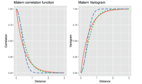
In practical modeling work we need to explicitly specify a particular covariance function so that the likelihood function can be written for the purposes of parameter estimation. In this section we discuss the most commonly used covariance function, namely the Matèrn family (Matérn, 1986) of covariance functions as an example of isotropic covariance functions. We discuss its special cases, such as the exponential and Gaussian. To proceed further recall from elementary definitions that covariance is simply variance times correlation if the two random variables (for which covariance is calculated) have the same variance. In spatial and spatio-temporal modeling, we assume equal spatial variance, which we denote by $\sigma^{2}$. Isotropic covariance functions depend on the distance between two locations, which we denote by $d$. Thus, the covariance function we are about to introduce will have the form
$$
C(d)=\sigma^{2} \rho(d), d>0
$$
where $\rho(d)$ is the correlation function. Note also that when $d=0$, the covariance is the same as the variance and should be equal to $\sigma^{2}$. Indeed, we shall assume that $\rho(d) \rightarrow 1$ as $d \rightarrow 0$. Henceforth we will only discuss covariance functions in the domain when $d>0$.

How should the correlation functions behave as the distance $d$ increases? For most natural and environmental processes, the correlation should decay with increasing $d$. Indeed, the Tobler’s first law of Geography (Tobler, 1970) states that, “everything is related to everything else, but near things are more related than distant things.” Indeed, there are stochastic processes where we may want to assume no correlation at all for any distance $d$ above a threshold value. Although this sounds very attractive and intuitively simple there are technical difficulties in modeling associated with this approach since an arbitrary covariance function may violate the requirement of non-negative definiteness of the variances. More about this requirement is discussed below in Section 2.7. There are mathematically valid ways to specify negligible amounts of correlations for large distances. See for example, the method of tapering discussed by Kaufman et al. (2008).

Usually, the correlation function $\rho(d)$ should monotonically decrease with increasing value of $d$ due to the Tobler’s law stated above. The particular value of $d$, say $d_{0}$, which is a solution of the equation $\rho(d)=0$ is called the range. This implies that the correlation is exactly zero between any two random observations observed at least the range $d_{0}$ distance apart. Note that due to the monotonicity of the correlation function, it cannot climb up once it reaches the value zero for some value of the distance $d$. With the added assumption of Gaussianity for the data, the range $d_{0}$ is the minimum distance beyond which any two random observations are deemed to be independent. With such assumptions we claim that the underlying process does not get affected by the same process, which is taking place at least $d_{0}$ distance away.

统计代写|贝叶斯统计代写beyesian statistics代考|Gaussian processes

Often Gaussian processes are assumed as components in spatial and spatiotemporal modeling. These stochastic processes are defined over a continuum, e.g. a spatial study region and specifying the resulting infinite dimensional random variable is often a challenge in practice. Gaussian processes are very convenient to work in these settings since they are fully defined by a mean function, say $\mu(\mathrm{s})$ and a valid covariance function, say $C\left(\left|\mathbf{s}-\mathbf{s}^{}\right|\right)=\operatorname{Cov}\left(Y(\mathbf{s}), Y\left(\mathbf{s}^{}\right)\right)$, which is required to be positive definite. A covariance function is said to be positive definite if the covariance matrix, implied by that covariance function, for a finite number of random variables belonging to that process is positive definite.

Suppose that the stochastic process $Y($ s ), defined over a continuous spatial region $\mathbb{D}$, is assumed to be a GP with mean function $\mu(\mathrm{s})$ and covariance function $C\left(\mathbf{s}, \mathbf{s}^{*}\right)$. Note that since $s$ is any point in $\mathbb{D}$, the process $Y$ (s) defines a non-countably infinite number of random variables. However, in practice

the GP assumption guarantees that for any finite $n$ and any set of $n$ locations $\mathbf{s}{1}, \ldots, \mathbf{s}{n}$ within $\mathbb{D}$ the $n$-variate random variable $\mathbf{Y}=\left(Y\left(\mathbf{s}{1}\right), \ldots, Y\left(\mathbf{s}{n}\right)\right)$ is normally distributed with mean $\boldsymbol{\mu}$ and covariance matrix $\Sigma$ given by:
$$
\boldsymbol{\mu}=\left(\begin{array}{c}
\mu\left(\mathbf{s}{1}\right) \ \mu\left(\mathbf{s}{2}\right) \
\vdots \
\mu\left(\mathbf{s}{n}\right) \end{array}\right), \quad \Sigma=\left(\begin{array}{cccc} C(0) & C\left(d{12}\right) & \cdots & C\left(d_{1 n}\right) \
C\left(d_{21}\right) & C(0) & \cdots & C\left(d_{2 n}\right) \
\vdots & \vdots & \ddots & \vdots \
C\left(d_{n 1}\right) & C\left(d_{n 2}\right) & \cdots & C(0)
\end{array}\right)
$$
where $d_{i j}=\left|\mathbf{s}{i}-\mathbf{s}{j}\right|$ is the distance between the two locations $\mathbf{s}{i}$ and $\mathbf{s}{j}$. From the multivariate normal distribution in Section A.1 in Appendix A, we can immediately write down the joint density of $\mathbf{Y}$ for any finite value of $n$. However, the unresolved matter is how do we specify the two functions $\mu\left(\mathbf{s}{i}\right)$ and $C\left(d{i j}\right)$ for any $i$ and $j$. The GP assumption is often made for the error process just as in usual regression modeling the error distribution is assumed to be Gaussian. Hence often a GP assumption comes with $\mu(\mathbf{s})=0$ for all s. The next most common assumption is to assume the Matèrn covariance function $C\left(d_{i j} \mid \psi\right)$ written down in $(2.1)$ for $C\left(d_{i j}\right)$. The Matèrn family provides a valid family of positive definite covariance functions, and it is the only family used in this book.

统计代写|贝叶斯统计代写Bayesian statistics代考|Isotropy

贝叶斯统计代写

统计代写|贝叶斯统计代写beyesian statistics代考|Isotropy

到目前为止,半变异函数C(H),或协方差函数C(H), 已假定依赖于多维H. 这是非常笼统且过于宽泛的,给建模者关于随机过程的巨大灵活性,因为它在空间域上变化,D. 然而,当过程从一个位置移动到下一个位置时,这种灵活性会带来很多负担,因为需要精确指定依赖结构。也就是说,函数C(H)需要为多维 h 的每个可能值指定。这不仅从模型规范的目的来看是有问题的,而且很难从数据中估计所有这些精确的特征。因此,引入了各向同性的概念以简化规范。

协方差函数C(H)如果仅取决于长度,则称其为各向同性的|H|分离向量的H. 各向同性协方差函数仅取决于距离,而不取决于行进的角度或方向。假设空间是二维的,各向同性协方差函数保证两个随机变量之间的协方差,一个在圆的中心,另一个在圆周上的任意点,与两个随机变量之间的协方差相同。中心和另一个在同一圆的圆周上的其他点。因此,协方差不取决于随机变量记录在圆周上的位置和方向。因此,这种协方差函数被称为全向的。

滥用符号一个各向同性的协方差函数,C(⋅)表示为C(|H|))或简单地通过C(d)在哪里d≥0是两个位置之间的标量距离。符号C(⋅)自从我们之前谈到的以来一直在这里被滥用C(H)在哪里H是一个多维分离向量,但现在一样C用于表示一维协方差函数C(d). 如果协方差函数不是各向同性的,则称为各向异性。

在实践中,各向同性协方差函数似乎过于严格,因为它们在不允许潜在随机过程的灵活协方差结构方面是刚性的。例如,污染羽流只能通过使用盛行风向传播,例如东西向。事实上,这是真的,而且通常各向同性的假设被视为建模工作的限制。然而,压倒性的简单性仍然胜过所有的缺点,并且各向同性协方差函数用于潜在的真实误差过程。许多数学结构和实用技巧用于构建各向异性协方差函数,例如参见 Banerjee 等人的第 3 章。(2015).

统计代写|贝叶斯统计代写beyesian statistics代考|Matèrn covariance function

在实际建模工作中,我们需要明确指定特定的协方差函数,以便可以编写似然函数以用于参数估计。在本节中,我们将讨论最常用的协方差函数,即协方差函数的 Matèrn 族 (Matérn, 1986),作为各向同性协方差函数的一个例子。我们讨论它的特殊情况,例如指数和高斯。从基本定义中进一步回忆,如果两个随机变量(为其计算协方差)具有相同的方差,则协方差只是方差乘以相关性。在空间和时空建模中,我们假设空间方差相等,我们表示为σ2. 各向同性协方差函数取决于两个位置之间的距离,我们表示为d. 因此,我们即将介绍的协方差函数将具有以下形式
C(d)=σ2ρ(d),d>0
在哪里ρ(d)是相关函数。另请注意,当d=0,协方差与方差相同,应等于σ2. 事实上,我们应该假设ρ(d)→1作为d→0. 以后我们将只讨论域中的协方差函数d>0.

相关函数应如何表现为距离d增加?对于大多数自然和环境过程,相关性应该随着增加而衰减d. 事实上,托布勒的第一地理定律(托布勒,1970 年)指出,“一切都与其他一切相关,但近处的事物比远处的事物更相关。” 确实,存在随机过程,我们可能希望假设任何距离都没有相关性d高于阈值。尽管这听起来非常有吸引力且直观简单,但与此方法相关的建模存在技术困难,因为任意协方差函数可能违反方差非负确定性的要求。下文第 2.7 节讨论了有关此要求的更多信息。有数学上有效的方法可以为大距离指定可忽略的相关量。例如,参见 Kaufman 等人讨论的锥形化方法。(2008 年)。

通常,相关函数ρ(d)应该随着值的增加而单调减少d由于上述托布勒定律。的特殊价值d, 说d0,这是方程的解ρ(d)=0称为范围。这意味着至少在范围内观察到的任何两个随机观测值之间的相关性恰好为零d0距离。请注意,由于相关函数的单调性,一旦达到某个距离值的零值,它就无法爬升d. 加上对数据的高斯假设,范围d0是任何两个随机观察被认为是独立的最小距离。有了这样的假设,我们声称底层过程不会受到相同过程的影响,至少正在发生d0距离。

统计代写|贝叶斯统计代写beyesian statistics代考|Gaussian processes

高斯过程通常被假定为空间和时空建模的组成部分。这些随机过程是在一个连续统一体上定义的,例如一个空间研究区域,并且指定生成的无限维随机变量在实践中通常是一个挑战。高斯过程在这些设置中工作非常方便,因为它们完全由平均函数定义,例如μ(s)和一个有效的协方差函数,比如说C(|s−s|)=这⁡(是(s),是(s)),它必须是正定的。如果协方差函数隐含的协方差矩阵对于属于该过程的有限数量的随机变量是正定的,则​​称协方差函数是正定的。

假设随机过程是(s ),定义在一个连续的空间区域上D, 假设为具有均值函数的 GPμ(s)和协方差函数C(s,s∗). 请注意,由于s是任何一点D, 过程是(s) 定义了不可数的无限数量的随机变量。然而,在实践中

GP 假设保证对于任何有限n和任何一组n地点s1,…,sn之内D这n- 变量随机变量是=(是(s1),…,是(sn))正态分布,均值μ和协方差矩阵Σ给出:
μ=(μ(s1) μ(s2) ⋮ μ(sn)),Σ=(C(0)C(d12)⋯C(d1n) C(d21)C(0)⋯C(d2n) ⋮⋮⋱⋮ C(dn1)C(dn2)⋯C(0))
在哪里d一世j=|s一世−sj|是两个位置之间的距离s一世和sj. 根据附录 A 中 A.1 节的多元正态分布,我们可以立即写下是对于任何有限值n. 但是,未解决的问题是我们如何指定这两个函数μ(s一世)和C(d一世j)对于任何一世和j. GP 假设通常用于误差过程,就像在通常的回归建模中假设误差分布是高斯分布一样。因此,通常伴随着 GP 假设μ(s)=0对于所有 s。下一个最常见的假设是假设 Matèrn 协方差函数C(d一世j∣ψ)写在(2.1)为了C(d一世j). Matèrn 族提供了一个有效的正定协方差函数族,它是本书中唯一使用的族。

统计代写|贝叶斯统计代写beyesian statistics代考 请认准statistics-lab™

统计代写请认准statistics-lab™. statistics-lab™为您的留学生涯保驾护航。

金融工程代写

金融工程是使用数学技术来解决金融问题。金融工程使用计算机科学、统计学、经济学和应用数学领域的工具和知识来解决当前的金融问题,以及设计新的和创新的金融产品。

非参数统计代写

非参数统计指的是一种统计方法,其中不假设数据来自于由少数参数决定的规定模型;这种模型的例子包括正态分布模型和线性回归模型。

广义线性模型代考

广义线性模型(GLM)归属统计学领域,是一种应用灵活的线性回归模型。该模型允许因变量的偏差分布有除了正态分布之外的其它分布。

术语 广义线性模型(GLM)通常是指给定连续和/或分类预测因素的连续响应变量的常规线性回归模型。它包括多元线性回归,以及方差分析和方差分析(仅含固定效应)。

有限元方法代写

有限元方法(FEM)是一种流行的方法,用于数值解决工程和数学建模中出现的微分方程。典型的问题领域包括结构分析、传热、流体流动、质量运输和电磁势等传统领域。

有限元是一种通用的数值方法,用于解决两个或三个空间变量的偏微分方程(即一些边界值问题)。为了解决一个问题,有限元将一个大系统细分为更小、更简单的部分,称为有限元。这是通过在空间维度上的特定空间离散化来实现的,它是通过构建对象的网格来实现的:用于求解的数值域,它有有限数量的点。边界值问题的有限元方法表述最终导致一个代数方程组。该方法在域上对未知函数进行逼近。[1] 然后将模拟这些有限元的简单方程组合成一个更大的方程系统,以模拟整个问题。然后,有限元通过变化微积分使相关的误差函数最小化来逼近一个解决方案。

tatistics-lab作为专业的留学生服务机构,多年来已为美国、英国、加拿大、澳洲等留学热门地的学生提供专业的学术服务,包括但不限于Essay代写,Assignment代写,Dissertation代写,Report代写,小组作业代写,Proposal代写,Paper代写,Presentation代写,计算机作业代写,论文修改和润色,网课代做,exam代考等等。写作范围涵盖高中,本科,研究生等海外留学全阶段,辐射金融,经济学,会计学,审计学,管理学等全球99%专业科目。写作团队既有专业英语母语作者,也有海外名校硕博留学生,每位写作老师都拥有过硬的语言能力,专业的学科背景和学术写作经验。我们承诺100%原创,100%专业,100%准时,100%满意。

随机分析代写


随机微积分是数学的一个分支,对随机过程进行操作。它允许为随机过程的积分定义一个关于随机过程的一致的积分理论。这个领域是由日本数学家伊藤清在第二次世界大战期间创建并开始的。

时间序列分析代写

随机过程,是依赖于参数的一组随机变量的全体,参数通常是时间。 随机变量是随机现象的数量表现,其时间序列是一组按照时间发生先后顺序进行排列的数据点序列。通常一组时间序列的时间间隔为一恒定值(如1秒,5分钟,12小时,7天,1年),因此时间序列可以作为离散时间数据进行分析处理。研究时间序列数据的意义在于现实中,往往需要研究某个事物其随时间发展变化的规律。这就需要通过研究该事物过去发展的历史记录,以得到其自身发展的规律。

回归分析代写

多元回归分析渐进(Multiple Regression Analysis Asymptotics)属于计量经济学领域,主要是一种数学上的统计分析方法,可以分析复杂情况下各影响因素的数学关系,在自然科学、社会和经济学等多个领域内应用广泛。

MATLAB代写

MATLAB 是一种用于技术计算的高性能语言。它将计算、可视化和编程集成在一个易于使用的环境中,其中问题和解决方案以熟悉的数学符号表示。典型用途包括:数学和计算算法开发建模、仿真和原型制作数据分析、探索和可视化科学和工程图形应用程序开发,包括图形用户界面构建MATLAB 是一个交互式系统,其基本数据元素是一个不需要维度的数组。这使您可以解决许多技术计算问题,尤其是那些具有矩阵和向量公式的问题,而只需用 C 或 Fortran 等标量非交互式语言编写程序所需的时间的一小部分。MATLAB 名称代表矩阵实验室。MATLAB 最初的编写目的是提供对由 LINPACK 和 EISPACK 项目开发的矩阵软件的轻松访问,这两个项目共同代表了矩阵计算软件的最新技术。MATLAB 经过多年的发展,得到了许多用户的投入。在大学环境中,它是数学、工程和科学入门和高级课程的标准教学工具。在工业领域,MATLAB 是高效研究、开发和分析的首选工具。MATLAB 具有一系列称为工具箱的特定于应用程序的解决方案。对于大多数 MATLAB 用户来说非常重要,工具箱允许您学习应用专业技术。工具箱是 MATLAB 函数(M 文件)的综合集合,可扩展 MATLAB 环境以解决特定类别的问题。可用工具箱的领域包括信号处理、控制系统、神经网络、模糊逻辑、小波、仿真等。

R语言代写问卷设计与分析代写
PYTHON代写回归分析与线性模型代写
MATLAB代写方差分析与试验设计代写
STATA代写机器学习/统计学习代写
SPSS代写计量经济学代写
EVIEWS代写时间序列分析代写
EXCEL代写深度学习代写
SQL代写各种数据建模与可视化代写

统计代写|贝叶斯统计代写Bayesian statistics代考|Jargon of spatial and spatio-temporal modeling

如果你也在 怎样代写贝叶斯统计这个学科遇到相关的难题,请随时右上角联系我们的24/7代写客服。

贝叶斯统计学是一个使用概率的数学语言来描述认识论的不确定性的系统。在 “贝叶斯范式 “中,对自然状态的相信程度是明确的;这些程度是非负的,而对所有自然状态的总相信是固定的。

statistics-lab™ 为您的留学生涯保驾护航 在代写贝叶斯统计方面已经树立了自己的口碑, 保证靠谱, 高质且原创的统计Statistics代写服务。我们的专家在代写贝叶斯统计代写方面经验极为丰富,各种代写贝叶斯统计相关的作业也就用不着说。

我们提供的贝叶斯统计及其相关学科的代写,服务范围广, 其中包括但不限于:

  • Statistical Inference 统计推断
  • Statistical Computing 统计计算
  • Advanced Probability Theory 高等概率论
  • Advanced Mathematical Statistics 高等数理统计学
  • (Generalized) Linear Models 广义线性模型
  • Statistical Machine Learning 统计机器学习
  • Longitudinal Data Analysis 纵向数据分析
  • Foundations of Data Science 数据科学基础
统计代写|贝叶斯统计代写Bayesian statistics代考|Jargon of spatial and spatio-temporal modeling

统计代写|贝叶斯统计代写beyesian statistics代考|Stochastic processes

We are familiar with the term random variable to denote measurements of outcomes of random experiments. For example, a random variable, say $Y$, could denote the height of a randomly chosen individual in a population of interest, such as a class of seven years old pupils in a primary school. If we

measure the height of $n$ randomly chosen children, then we denote these heights by notations $y_{1}, \ldots, y_{n}$ which are the recorded numerical values. We use the corresponding upper case letters $Y_{1}, \ldots, Y_{n}$ to denote the physical random variable: heights of $n$ randomly selected children.

The concept of random variables is sound and adequate enough when we intend to model and analyze data which are not associated with a continuous domain. For example, the population of seven years old is countable and finite – so the associated domain is not continuous. Further examples include hourly air pollution values recorded at the top of the hour at a particular monitoring site within a city. However, this concept of random variables is not adequate enough when we allow the possibility of having an uncountably infinite collection of random variables associated with a continuous domain such as space or time, or both. For example, suppose that we are interested in modeling an air pollution surface over a city. Because the spatial domain is continuous here, having an uncountably infinite number of locations, we shall require a richer concept of uncountably infinite number of random variables. Hence, we welcome the arrival of the concept of stochastic processes.

A stochastic process is an uncountably infinite collection of random variables defined on a continuous domain such as space, time, or both. Hence, the discrete notation, $Y_{i}, i=1,2, \ldots$ for random variables is changed to either $Y(\mathbf{s}), Y(t)$ or $Y(\mathbf{s}, t)$ where $s$ denotes a spatial location, described by a finite number of dimensions such as latitude, longitude, altitude, etc. and $t$ denotes a continuously measured time point depending on the data collection situation: only spatial, only temporal, and spatio-temporal, respectively. In the spatial only case, we shall use $Y($ s ) to denote a spatial stochastic process or simply a spatial process defined over a domain $\mathbb{D}$, say. In the temporal only case, $Y(t)$ is used to denote the temporally varying stochastic process over a continuous time period, $0 \leq t \leq T$. When time is considered to be discrete, e.g. hourly, then it is notationally convenient to use the notation $Y_{t}$ instead of the more general $Y(t)$. In this case, $Y_{t}$ is better referred to as a time series.

In this book we shall not consider time in the continuous domain at all since such analyses are much more theoretically rich, requiring deeper theoretical understanding but practically not so common in the subject area of the examples described previously in Chapter 1 . Henceforth, we will use the notation $t$ to denote time in a discrete sense and domain. With $t$ being discrete, which of the two notations: $Y(\mathbf{s}, t)$ and $Y_{t}(\mathbf{s})$, should be adopted to denote our spatio-temporal data? Both the notations make sense, and it will be perfectly fine to use either. In this book we adopt the first, slightly more elaborate, notation $Y(s, t)$ throughout, although the subscript $t$ will be used to denote vector-valued random variables as necessary. Hence, the notation $y(\mathbf{s}, t)$ will denote a realization of a spatial stochastic process at location s and at a discrete-time point $t$.

统计代写|贝叶斯统计代写beyesian statistics代考|Stationarity

An object is stationary if it does not move from a fixed position. To be stationary, a stochastic process must possess certain stable behavior. A stochastic process, constituting of an infinite collection of random variables, cannot be a constant everywhere since otherwise, it will not be stochastic at all. Hence it makes sense to define stationarity of particular properties, e.g. mean and variance. The type of stationarity depends on the stationarity of the particular property of the stochastic process. In the discussion below, and throughout, we shall assume that the stochastic process under consideration has finite mean and variance, respectively denoted by $\mu(\mathbf{s})$ and $V(\mathbf{s})$ for all values of $s$ in $\mathbb{D}$.
A stochastic process, $Y(\mathbf{s})$, is said to be mean stationary if its mean is constant over the whole domain $\mathbb{D}$. For a mean stationary process $Y(\mathbf{s})$, $\mu(\mathbf{s})=E(Y(\mathbf{s}))$ is a constant function of s. Thus, the mean surface of a mean stationary stochastic process will imply a one-color map depicting the mean over the domain $\mathbb{D}$. Such a map will not exhibit any spatial trend in any direction. Note that this does not mean that a particular realization of the stochastic process, $Y(s)$ at $n$ locations $\mathbf{s}{1}, \mathbf{s}{2}, \ldots, \mathbf{s}{n}$ will yield a constant surface, $y\left(\mathbf{s}{1}\right)=y\left(\mathbf{s}{2}\right)=\ldots=y\left(\mathbf{s}{n}\right)$. Rather, mean stationarity of a process $Y(\mathbf{s})$ means that $\mu\left(\mathbf{s}{1}\right)=\mu\left(\mathbf{s}{2}\right)=\cdots=\mu\left(\mathbf{s}{n}\right)$ at an arbitrary set of $n$ locations, $\mathbf{s}{1}, \mathbf{s}{2}, \ldots, \mathbf{s}{n}$, where $n$ itself is an arbitrary positive integer. Similarly, we say that a time series, $Y_{t}$ is mean stationary if $E\left(Y_{t}\right),\left(=\mu_{t}\right.$, say), does not depend on the value of $t$. A mean stationary process is rarely of interest since, often, the main interest of the study is to investigate spatial and/or temporal variation. However, we often assume a zero-mean stationary process for the underlying error distribution or a prior process in modeling.

In spatial and temporal investigations often it is of interest to study the relationships, described by covariance or correlation, between the random variables at different locations. For example, one may ask, “will the covariance between two random variables at two different locations depend on the two locations as well as the distance between the two?” A lot of simplification in analysis is afforded when it is assumed that the covariance only depends on the simple difference (given by the separation vector $\mathbf{s}-\mathbf{s}^{\prime},=\mathbf{h}$, say) between two locations $s$ and $\mathbf{s}^{\prime}$ and not on the actual locations $\mathbf{s}$ and $\mathbf{s}^{\prime}$. A stochastic process $Y(\mathbf{s})$ is said to be covariance stationary if $\operatorname{Cov}\left(Y(\mathbf{s}), Y\left(\mathbf{s}^{\prime}\right)\right)=C(\mathbf{h})$ where $C$ is a suitable function of the difference $\mathbf{h}$. The function $C(\mathbf{h})$ is called the covariance function of the stochastic process and plays a crucial role in many aspects of spatial analysis. The global nature of the covariance function $C(\mathbf{h})$, as it is free of any particular location in the domain $\mathbb{D}$, helps

tremendously to simplify modeling and analysis and to specify joint distributions for the underlying random variables.

A stochastic process, $Y(\mathrm{~s})$, is said to be variance stationary if its variance, $V(\mathbf{s})$, is a constant, say $\sigma^{2}$, over the whole domain $\mathbb{D}$. For a variance stationary process, no heterogeneity arises due to variation either in space or time. This is again a very strong assumption that may not hold in practice. However, while modeling we often assume that the underlying error distribution has a constant spatial variance. Other methods and tricks, such as data transformation and amalgamation of several processes are employed to model non-constant spatial variance.

统计代写|贝叶斯统计代写beyesian statistics代考|Variogram and covariogram

The quantity $\operatorname{Var}(Y(\mathbf{s}+\mathbf{h})-Y(\mathbf{s}))$ is called the variogram of the stochastic process, $Y$ (s) as it measures the variance of the first difference in the process at two different locations $\mathbf{s}+\mathbf{h}$ and $\mathbf{s}$. Our desire for a simplified analysis,

using intrinsic stationarity, would dictate us to suppose that the variogram depends only on the separation vector $h$ and not on the actual location $\mathbf{s}$.
There is a one-to-one relationship between the variogram under the assumption of mean and variance stationarity for a process $Y(\mathbf{s})$. Assuming mean and variance stationary we have $E(Y(\mathbf{s}+\mathbf{h}))=E(Y(\mathbf{s}))$ and $\operatorname{Var}(Y(\mathbf{s}+\mathbf{h}))=\operatorname{Var}(Y(\mathbf{s}))=C(\mathbf{0})$, the spatial variance. For an intrinsically stationary process, we have:
$$
\begin{aligned}
\operatorname{Var}(Y(\mathbf{s}+\mathbf{h})-Y(\mathbf{s})) &=E{Y(\mathbf{s}+\mathbf{h})-Y(\mathbf{s})-E(Y(\mathbf{s}+\mathbf{h})+Y(\mathbf{s}))}^{2} \
&=E{(Y(\mathbf{s}+\mathbf{h})-E(Y(\mathbf{s}+\mathbf{h})))-(Y(\mathbf{s})-E(Y(\mathbf{s})))}^{2} \
&=E\left{(Y(\mathbf{s}+\mathbf{h})-E(Y(\mathbf{s}+\mathbf{h})))^{2}\right}+E\left{(Y(\mathbf{s})-E(Y(\mathbf{s})))^{2}\right} \
&=-2 E{(Y(\mathbf{s}+\mathbf{h})-E(Y(\mathbf{s}+\mathbf{h})))(Y(\mathbf{s})-E(Y(\mathbf{s})))} \
&=C(\mathbf{0}(Y(\mathbf{s}+\mathbf{h}))+\operatorname{Var}(Y(\mathbf{s}))-2 \operatorname{Cov}(Y(\mathbf{s}+\mathbf{h}), Y(\mathbf{s}))-2 C(\mathbf{h})\
&=2(C(\mathbf{0})-C(\mathbf{h})) .
\end{aligned}
$$
This result states that:
Variogram at separation $\mathbf{h}=2 \times{$ Spatial variance $-$ Spatial covariance function at separation $\mathbf{h}}$.

Clearly, we can easily find the variogram if we already have a specification for the spatial covariance function for all values of its argument. However, it is not easy to retrieve the covariance function from a specification of the variogram function, $\operatorname{Var}(Y(\mathbf{s}+\mathbf{h})-Y(\mathbf{s}))$. This needs further assumptions and limiting arguments, see e.g. Chapter 2 of Banerjee et al. (2015).

In order to study the behavior of a variogram, $2(C(\mathbf{0})-C(\mathbf{h}))$, as a function of the covariance function $C(\mathbf{h})$, we see that the multiplicative factor 2 is only a distraction. This is why, the semi-variogram, which is half of the variogram is conventionally studied in the literature. We use the notation $\gamma(\mathbf{h})$ to denote the semi-variogram, and thus $\gamma(\mathbf{h})=C(\mathbf{0})-C(\mathbf{h})$.

In practical modeling work we assume a specific valid covariance function $C(\mathbf{h})$ for the stochastic process and then the semi-variogram, $\gamma(\mathbf{h})$ is automatically determined. The word “valid” has been included in the previous sentence since a positive definiteness condition is required to ensure nonnegativeness of variances of all possible linear combinations of the random variables $Y\left(\mathbf{s}{1}\right), \ldots, Y\left(\mathbf{s}{n}\right)$. The simplification provided by the assumption of intrinsic stationarity is still not enough for practical modeling work since it is still very hard to specify a valid multi-dimensional function $C(\mathbf{h})$ as a function of the separation vector $\mathbf{h}$. The crucial concept of isotropy, defined and discussed below, accomplishes this task of specifying the covariance function as a one-dimensional function.

统计代写|贝叶斯统计代写Bayesian statistics代考|Jargon of spatial and spatio-temporal modeling

贝叶斯统计代写

统计代写|贝叶斯统计代写beyesian statistics代考|Stochastic processes

我们熟悉术语随机变量来表示随机实验结果的测量。例如,一个随机变量,比如说是, 可以表示在感兴趣的人群中随机选择的个体的身高,例如小学中一个七岁学生的班级。要是我们

测量高度n随机选择的孩子,然后我们用符号表示这些高度是1,…,是n这是记录的数值。我们使用对应的大写字母是1,…,是n表示物理随机变量:高度n随机选择的孩子。

当我们打算对与连续域无关的数据进行建模和分析时,随机变量的概念是合理且足够的。例如,七岁的人口是可数的和有限的——因此相关域不是连续的。进一步的例子包括在城市内特定监测点的每小时顶部记录的每小时空气污染值。然而,当我们允许拥有与空间或时间等连续域相关联的随机变量的无限集合的可能性时,这个随机变量的概念是不够的,或两者兼而有之。例如,假设我们对模拟城市上空的空气污染表面感兴趣。因为这里的空间域是连续的,有无数个位置,我们将需要一个更丰富的概念,即不可数无限的随机变量。因此,我们欢迎随机过程概念的到来。

随机过程是在空间、时间或两者兼有的连续域上定义的不可数无限的随机变量集合。因此,离散符号,是一世,一世=1,2,…对于随机变量更改为是(s),是(吨)或者是(s,吨)在哪里s表示空间位置,由有限数量的维度描述,例如纬度、经度、高度等,并且吨表示取决于数据收集情况的连续测量时间点:分别为仅空间、仅时间和时空。在仅空间的情况下,我们将使用是(s ) 表示空间随机过程或简单地定义在域上的空间过程D, 说。在时间唯一的情况下,是(吨)用于表示在连续时间段内随时间变化的随机过程,0≤吨≤吨. 当时间被认为是离散的,例如每小时,那么使用符号在符号上很方便是吨而不是更一般的是(吨). 在这种情况下,是吨更好地称为时间序列。

在本书中,我们根本不会考虑连续域中的时间,因为这样的分析在理论上要丰富得多,需要更深入的理论理解,但实际上在第 1 章前面描述的示例的主题领域中并不常见。此后,我们将使用符号吨以离散的意义和领域表示时间。和吨是离散的,两种表示法中的哪一种:是(s,吨)和是吨(s), 应该用来表示我们的时空数据吗?这两种表示法都有意义,使用任何一种都可以。在本书中,我们采用了第一个稍微复杂一点的符号是(s,吨)通篇,虽然下标吨必要时将用于表示向量值随机变量。因此,符号是(s,吨)将表示在位置 s 和离散时间点的空间随机过程的实现吨.

统计代写|贝叶斯统计代写beyesian statistics代考|Stationarity

如果物体不从固定位置移动,则它是静止的。为了保持平稳,随机过程必须具有一定的稳定行为。由无限随机变量集合构成的随机过程不可能在任何地方都是常数,否则它根本就不是随机的。因此,定义特定属性的平稳性是有意义的,例如均值和方差。平稳性的类型取决于随机过程的特定属性的平稳性。在下面的讨论中,我们将假设所考虑的随机过程具有有限的均值和方差,分别表示为μ(s)和在(s)对于所有值s在D.
一个随机过程,是(s),如果其均值在整个域上是恒定的,则称其为均值平稳的D. 对于平均平稳过程是(s), μ(s)=和(是(s))是 s 的常数函数。因此,平均平稳随机过程的平均表面将意味着一个单色图描绘了域上的平均值D. 这样的地图在任何方向都不会表现出任何空间趋势。请注意,这并不意味着随机过程的特定实现,是(s)在n地点s1,s2,…,sn将产生一个恒定的表面,是(s1)=是(s2)=…=是(sn). 相反,意味着过程的平稳性是(s)意思是μ(s1)=μ(s2)=⋯=μ(sn)在任意一组n地点,s1,s2,…,sn, 在哪里n本身是一个任意的正整数。同样,我们说一个时间序列,是吨是平均平稳的,如果和(是吨),(=μ吨, 说), 不依赖于吨. 平均平稳过程很少受到关注,因为该研究的主要兴趣通常是研究空间和/或时间变化。但是,我们经常假设潜在误差分布的零均值平稳过程或建模中的先前过程。

在空间和时间研究中,研究不同位置的随机变量之间的关系(由协方差或相关性描述)通常是有意义的。例如,有人可能会问,“两个不同位置的两个随机变量之间的协方差是否取决于这两个位置以及两者之间的距离?” 当假设协方差仅取决于简单的差异(由分离向量给出s−s′,=H, 说) 在两个位置之间s和s′而不是在实际位置s和s′. 随机过程是(s)据说是协方差平稳的,如果这⁡(是(s),是(s′))=C(H)在哪里C是差的合适函数H. 功能C(H)被称为随机过程的协方差函数,在空间分析的许多方面都起着至关重要的作用。协方差函数的全局性质C(H),因为它在域中没有任何特定位置D, 帮助

极大地简化了建模和分析,并指定了基础随机变量的联合分布。

一个随机过程,是( s),如果其方差,则称其为方差平稳的,在(s), 是一个常数,比如说σ2, 在整个域上D. 对于方差平稳过程,不会因空间或时间的变化而出现异质性。这又是一个非常强的假设,在实践中可能不成立。然而,在建模时,我们经常假设潜在的误差分布具有恒定的空间方差。其他方法和技巧,例如数据转换和多个过程的合并,用于模拟非恒定空间方差。

统计代写|贝叶斯统计代写beyesian statistics代考|Variogram and covariogram

数量曾是⁡(是(s+H)−是(s))称为随机过程的变异函数,是(s) 因为它测量两个不同位置的过程中的第一个差异的方差s+H和s. 我们渴望简化分析,

使用内在平稳性,将要求我们假设变异函数仅取决于分离向量H而不是在实际位置s.
在过程的均值和方差平稳性假设下,变异函数之间存在一对一的关系是(s). 假设均值和方差是固定的,我们有和(是(s+H))=和(是(s))和曾是⁡(是(s+H))=曾是⁡(是(s))=C(0),空间方差。对于本质上平稳的过程,我们有:
\begin{aligned} \operatorname{Var}(Y(\mathbf{s}+\mathbf{h})-Y(\mathbf{s})) &=E{Y(\mathbf{s}+\mathbf{ h})-Y(\mathbf{s})-E(Y(\mathbf{s}+\mathbf{h})+Y(\mathbf{s}))}^{2} \ &=E{( Y(\mathbf{s}+\mathbf{h})-E(Y(\mathbf{s}+\mathbf{h})))-(Y(\mathbf{s})-E(Y(\mathbf {s})))}^{2} \ &=E\left{(Y(\mathbf{s}+\mathbf{h})-E(Y(\mathbf{s}+\mathbf{h}) ))^{2}\right}+E\left{(Y(\mathbf{s})-E(Y(\mathbf{s})))^{2}\right} \ &=-2 E{ (Y(\mathbf{s}+\mathbf{h})-E(Y(\mathbf{s}+\mathbf{h})))(Y(\mathbf{s})-E(Y(\mathbf {s})))} \ &=C(\mathbf{0}(Y(\mathbf{s}+\mathbf{h}))+\operatorname{Var}(Y(\mathbf{s}))- 2 \operatorname{Cov}(Y(\mathbf{s}+\mathbf{h}), Y(\mathbf{s}))-2 C(\mathbf{h})\ &=2(C(\mathbf {0})-C(\mathbf{h})) .\end{aligned}\begin{aligned} \operatorname{Var}(Y(\mathbf{s}+\mathbf{h})-Y(\mathbf{s})) &=E{Y(\mathbf{s}+\mathbf{ h})-Y(\mathbf{s})-E(Y(\mathbf{s}+\mathbf{h})+Y(\mathbf{s}))}^{2} \ &=E{( Y(\mathbf{s}+\mathbf{h})-E(Y(\mathbf{s}+\mathbf{h})))-(Y(\mathbf{s})-E(Y(\mathbf {s})))}^{2} \ &=E\left{(Y(\mathbf{s}+\mathbf{h})-E(Y(\mathbf{s}+\mathbf{h}) ))^{2}\right}+E\left{(Y(\mathbf{s})-E(Y(\mathbf{s})))^{2}\right} \ &=-2 E{ (Y(\mathbf{s}+\mathbf{h})-E(Y(\mathbf{s}+\mathbf{h})))(Y(\mathbf{s})-E(Y(\mathbf {s})))} \ &=C(\mathbf{0}(Y(\mathbf{s}+\mathbf{h}))+\operatorname{Var}(Y(\mathbf{s}))- 2 \operatorname{Cov}(Y(\mathbf{s}+\mathbf{h}), Y(\mathbf{s}))-2 C(\mathbf{h})\ &=2(C(\mathbf {0})-C(\mathbf{h})) .\end{aligned}
该结果表明:
分离时的变异函数H=2×$小号p一种吨一世一种l在一种r一世一种nC和$−$小号p一种吨一世一种lC这在一种r一世一种nC和F在nC吨一世这n一种吨s和p一种r一种吨一世这n$H.

显然,如果我们已经为它的参数的所有值指定了空间协方差函数的规范,我们可以很容易地找到变异函数。但是,从变差函数的规范中检索协方差函数并不容易,曾是⁡(是(s+H)−是(s)). 这需要进一步的假设和限制性论据,例如参见 Banerjee 等人的第 2 章。(2015 年)。

为了研究变异函数的行为,2(C(0)−C(H)), 作为协方差函数的函数C(H),我们看到乘法因子 2 只是一种干扰。这就是为什么在文献中通常研究半变异函数,它是变异函数的一半。我们使用符号C(H)表示半变异函数,因此C(H)=C(0)−C(H).

在实际建模工作中,我们假设一个特定的有效协方差函数C(H)对于随机过程,然后是半变异函数,C(H)是自动确定的。上一句中包含了“有效”一词,因为需要一个正定条件来确保随机变量的所有可能线性组合的方差的非负性是(s1),…,是(sn). 内在平稳性假设所提供的简化对于实际建模工作仍然不够,因为仍然很难指定有效的多维函数C(H)作为分离向量的函数H. 下面定义和讨论的各向同性的关键概念完成了将协方差函数指定为一维函数的任务。

统计代写|贝叶斯统计代写beyesian statistics代考 请认准statistics-lab™

统计代写请认准statistics-lab™. statistics-lab™为您的留学生涯保驾护航。

金融工程代写

金融工程是使用数学技术来解决金融问题。金融工程使用计算机科学、统计学、经济学和应用数学领域的工具和知识来解决当前的金融问题,以及设计新的和创新的金融产品。

非参数统计代写

非参数统计指的是一种统计方法,其中不假设数据来自于由少数参数决定的规定模型;这种模型的例子包括正态分布模型和线性回归模型。

广义线性模型代考

广义线性模型(GLM)归属统计学领域,是一种应用灵活的线性回归模型。该模型允许因变量的偏差分布有除了正态分布之外的其它分布。

术语 广义线性模型(GLM)通常是指给定连续和/或分类预测因素的连续响应变量的常规线性回归模型。它包括多元线性回归,以及方差分析和方差分析(仅含固定效应)。

有限元方法代写

有限元方法(FEM)是一种流行的方法,用于数值解决工程和数学建模中出现的微分方程。典型的问题领域包括结构分析、传热、流体流动、质量运输和电磁势等传统领域。

有限元是一种通用的数值方法,用于解决两个或三个空间变量的偏微分方程(即一些边界值问题)。为了解决一个问题,有限元将一个大系统细分为更小、更简单的部分,称为有限元。这是通过在空间维度上的特定空间离散化来实现的,它是通过构建对象的网格来实现的:用于求解的数值域,它有有限数量的点。边界值问题的有限元方法表述最终导致一个代数方程组。该方法在域上对未知函数进行逼近。[1] 然后将模拟这些有限元的简单方程组合成一个更大的方程系统,以模拟整个问题。然后,有限元通过变化微积分使相关的误差函数最小化来逼近一个解决方案。

tatistics-lab作为专业的留学生服务机构,多年来已为美国、英国、加拿大、澳洲等留学热门地的学生提供专业的学术服务,包括但不限于Essay代写,Assignment代写,Dissertation代写,Report代写,小组作业代写,Proposal代写,Paper代写,Presentation代写,计算机作业代写,论文修改和润色,网课代做,exam代考等等。写作范围涵盖高中,本科,研究生等海外留学全阶段,辐射金融,经济学,会计学,审计学,管理学等全球99%专业科目。写作团队既有专业英语母语作者,也有海外名校硕博留学生,每位写作老师都拥有过硬的语言能力,专业的学科背景和学术写作经验。我们承诺100%原创,100%专业,100%准时,100%满意。

随机分析代写


随机微积分是数学的一个分支,对随机过程进行操作。它允许为随机过程的积分定义一个关于随机过程的一致的积分理论。这个领域是由日本数学家伊藤清在第二次世界大战期间创建并开始的。

时间序列分析代写

随机过程,是依赖于参数的一组随机变量的全体,参数通常是时间。 随机变量是随机现象的数量表现,其时间序列是一组按照时间发生先后顺序进行排列的数据点序列。通常一组时间序列的时间间隔为一恒定值(如1秒,5分钟,12小时,7天,1年),因此时间序列可以作为离散时间数据进行分析处理。研究时间序列数据的意义在于现实中,往往需要研究某个事物其随时间发展变化的规律。这就需要通过研究该事物过去发展的历史记录,以得到其自身发展的规律。

回归分析代写

多元回归分析渐进(Multiple Regression Analysis Asymptotics)属于计量经济学领域,主要是一种数学上的统计分析方法,可以分析复杂情况下各影响因素的数学关系,在自然科学、社会和经济学等多个领域内应用广泛。

MATLAB代写

MATLAB 是一种用于技术计算的高性能语言。它将计算、可视化和编程集成在一个易于使用的环境中,其中问题和解决方案以熟悉的数学符号表示。典型用途包括:数学和计算算法开发建模、仿真和原型制作数据分析、探索和可视化科学和工程图形应用程序开发,包括图形用户界面构建MATLAB 是一个交互式系统,其基本数据元素是一个不需要维度的数组。这使您可以解决许多技术计算问题,尤其是那些具有矩阵和向量公式的问题,而只需用 C 或 Fortran 等标量非交互式语言编写程序所需的时间的一小部分。MATLAB 名称代表矩阵实验室。MATLAB 最初的编写目的是提供对由 LINPACK 和 EISPACK 项目开发的矩阵软件的轻松访问,这两个项目共同代表了矩阵计算软件的最新技术。MATLAB 经过多年的发展,得到了许多用户的投入。在大学环境中,它是数学、工程和科学入门和高级课程的标准教学工具。在工业领域,MATLAB 是高效研究、开发和分析的首选工具。MATLAB 具有一系列称为工具箱的特定于应用程序的解决方案。对于大多数 MATLAB 用户来说非常重要,工具箱允许您学习应用专业技术。工具箱是 MATLAB 函数(M 文件)的综合集合,可扩展 MATLAB 环境以解决特定类别的问题。可用工具箱的领域包括信号处理、控制系统、神经网络、模糊逻辑、小波、仿真等。

R语言代写问卷设计与分析代写
PYTHON代写回归分析与线性模型代写
MATLAB代写方差分析与试验设计代写
STATA代写机器学习/统计学习代写
SPSS代写计量经济学代写
EVIEWS代写时间序列分析代写
EXCEL代写深度学习代写
SQL代写各种数据建模与可视化代写

统计代写|贝叶斯统计代写Bayesian statistics代考|Areal unit data sets used in the book

如果你也在 怎样代写贝叶斯统计这个学科遇到相关的难题,请随时右上角联系我们的24/7代写客服。

贝叶斯统计学是一个使用概率的数学语言来描述认识论的不确定性的系统。在 “贝叶斯范式 “中,对自然状态的相信程度是明确的;这些程度是非负的,而对所有自然状态的总相信是固定的。

statistics-lab™ 为您的留学生涯保驾护航 在代写贝叶斯统计方面已经树立了自己的口碑, 保证靠谱, 高质且原创的统计Statistics代写服务。我们的专家在代写贝叶斯统计代写方面经验极为丰富,各种代写贝叶斯统计相关的作业也就用不着说。

我们提供的贝叶斯统计及其相关学科的代写,服务范围广, 其中包括但不限于:

  • Statistical Inference 统计推断
  • Statistical Computing 统计计算
  • Advanced Probability Theory 高等概率论
  • Advanced Mathematical Statistics 高等数理统计学
  • (Generalized) Linear Models 广义线性模型
  • Statistical Machine Learning 统计机器学习
  • Longitudinal Data Analysis 纵向数据分析
  • Foundations of Data Science 数据科学基础
统计代写|贝叶斯统计代写Bayesian statistics代考|Areal unit data sets used in the book

统计代写|贝叶斯统计代写beyesian statistics代考|Covid-19 mortality data from England

This data set presents the number of deaths due to Covid- 19 during the peak from March 13 to July 31,2020 in the 313 Local Authority Districts, Counties and Unitary Authorities (LADCUA) in England; see Figure 1.8. There are 49,292 weekly recorded deaths during this period of 20 weeks. Figure $1.9$ shows a map of the number of deaths and the death rate per 100,000 people in each of the 313 LADCUAs. Contrasting the two plots, it is clear that much spatial variation is seen in the right panel of the death rates per 100,000 people. The boxplot of the weekly death rates shown in Figure $1.10$ shows the first peak during weeks 15 and 16 (April 10th to 23 rd) and a very slow decline of the death numbers after the peak. The main purpose here is to model the spatiotemporal variation in the death rates. This data set will be used as a running example for all the areal unit data models in Chapter 10. Chapter 3 provides some further preliminary exploratory analysis of this data set.

The Demographic and Health Surveys (DHS) program ${ }^{1}$ routinely collects several data sets for monitoring health at a global level. This example is based on a 2014 vaccination coverage data set for the country Kenya in East Africa. The data set contains the number of children aged 12-23 months who had received the first dose of measles-containing vaccine (MCV1) at any time before the survey in 2014. Figure $1.11$ plots the observed vaccination proportions in 2014. A substantial analysis of this and several related data sets has been conducted by Utazi et al. (2021). Modeled in Section 11.2, this example aims to assess vaccination coverage rates in the different counties in Kenya.

统计代写|贝叶斯统计代写beyesian statistics代考|Cancer rates in the United States

The Centers for Disease Control and Prevention in the United States provides downloadable cancer rate data at various geographical levels, e.g. the 50 states. Such a data set can be downloaded along with various information e.g. gender and ethnicity and types of cancer. However, due to the data identifiability and data protection reasons, some of the smaller rate counts (which arises due to finer classification by the factors) rates are not made public. Hence, for the purposes of illustration of this book, we aim to model aggregated annual data at the state level. The full data set provides state-wise annual rates of cancer from all causes during from 2003 to 2017 . Figure $1.12$ provides a map of the aggregated cancer rates per 100,000 people from all causes during from 2003 to 2017 for the 48 contiguous states. This is an example of a choropleth map that uses shades of color or gray scale to classify values into a few broad classes, like a histogram. The figure shows higher total incidence rates in the northeast compared to south-west. Florida also shows a higher rate which may be attributed to a larger share of the retired elderly residents in the state. The full spatio-temporal data set will be analyzed in Section 11.3.

The observed standardized mortality rates, see discussion in Section $11.3$ on how to obtain those, for ten selected states are shown in Figure 1.13. These states are hand-picked to represent the full range of the SMR values. The research question that is of interest here is, “is there an upward trend in these rates after accounting for spatio-temporal correlation and any other important fixed effects covariates?” This is investigated in Section 11.3.

统计代写|贝叶斯统计代写beyesian statistics代考|Hospitalization data from England

Monthly counts of the numbers of hospitalizations due to respiratory diseases from the 323 Local and Unitary Authorities (LUA) in England for the 60 months in the 5 -year period 2007 to 2011 are available from the study published by Lee et al. (2017). These counts depend on the size and demographics of the population at risk, which are adjusted for by computing the expected number of hospital admissions $E_{i t}$ using what is known as indirect standardization, see Section $2.12$, from national age and sex-specific hospitalization rates in England.

In this example, the study region is England, UK, partitioned into $i=$ $1, \ldots, n=323$ Local and Unitary Authorities (LUA), and data are available for $t=1, \ldots, T=60$ months between 2007 and 2011 . Counts of the numbers of respiratory hospitalizations for LUA $i$ and month $t$ are denoted by $Y_{i t}$, for $i=1, \ldots, 323$ and $t=1, \ldots, 60$, which have a median value of 111 and a range from 6 to 2485 . The monthly time scale matches the study by Greven et al. (2011), whereas the majority of studies such as Lee et al. (2009) utilize yearly data. An advantage of the monthly scale is that it requires less aggregation of the data away from the individual level, but it does mean that $Y_{\text {it }}$ could include admissions driven by both chronic and acute pollution exposure.
The spatial (left panel) and temporal (bottom panel) patterns in the Standardized Morbidity Ratio, $\mathrm{SMR}{i t}=Y{i t} / E_{\text {it }}$ are displayed in Figure $1.14$, where a value of $1.2$ corresponds to a $20 \%$ increased risk compared to $E_{i t}$. The figure shows the highest risks are in cities in the center and north of England, such as Birmingham, Leeds and Manchester, while the temporal pattern is strongly seasonal, with higher risks of admission in the winter due to factors such as influenza epidemics and cold temperature. This data set is used as an example in Section $11.4$ of this book.

统计代写|贝叶斯统计代写Bayesian statistics代考|Areal unit data sets used in the book

贝叶斯统计代写

统计代写|贝叶斯统计代写beyesian statistics代考|Covid-19 mortality data from England

该数据集显示了 2020 年 3 月 13 日至 7 月 31 日高峰期间英格兰 313 个地方当局区、县和单一当局 (LADCUA) 因 Covid-19 导致的死亡人数;见图 1.8。在这 20 周期间,每周记录的死亡人数为 49,292 人。数字1.9显示了 313 个 LADCUA 中每一个的死亡人数和每 100,000 人死亡率的地图。对比这两个图,很明显,在每 100,000 人的死亡率右侧面板中可以看到很大的空间变化。每周死亡率的箱线图如图所示1.10显示第 15 周和第 16 周(4 月 10 日至 23 日)的第一个高峰,高峰后死亡人数的下降非常缓慢。这里的主要目的是模拟死亡率的时空变化。该数据集将用作第 10 章中所有区域单元数据模型的运行示例。第 3 章对该数据集进行了一些进一步的初步探索性分析。

人口与健康调查 (DHS) 计划1定期收集多个数据集以在全球范围内监测健康状况。此示例基于 2014 年东非肯尼亚国家的疫苗接种覆盖率数据集。该数据集包含在 2014 年调查之前的任何时间接种过第一剂麻疹疫苗 (MCV1) 的 12-23 个月大的儿童人数。 图1.11绘制了 2014 年观察到的疫苗接种比例。Utazi 等人对此和几个相关数据集进行了实质性分析。(2021 年)。本示例在第 11.2 节中建模,旨在评估肯尼亚不同县的疫苗接种覆盖率。

统计代写|贝叶斯统计代写beyesian statistics代考|Cancer rates in the United States

美国疾病控制和预防中心提供不同地理级别(例如 50 个州)的可下载癌症发病率数据。这样的数据集可以与各种信息一起下载,例如性别、种族和癌症类型。但是,由于数据可识别性和数据保护的原因,一些较小的费率计数(由于因素分类更精细而产生)并未公开。因此,为了说明本书的目的,我们的目标是在州一级对汇总的年度数据进行建模。完整的数据集提供了从 2003 年到 2017 年各州各种原因的癌症年发病率。数字1.12提供了 2003 年至 2017 年期间 48 个相邻州的每 10 万人中各种原因的总癌症发病率地图。这是一个等值线图示例,它使用颜色或灰度的阴影将值分类为几个大类,如直方图。该图显示,与西南相比,东北的总发病率更高。佛罗里达州也显示出更高的比率,这可能归因于该州退休老年居民的比例更大。完整的时空数据集将在 11.3 节中进行分析。

观察到的标准化死亡率,见章节中的讨论11.3关于如何获得这些,对于十个选定的状态,如图 1.13 所示。这些状态是精心挑选的,以代表 SMR 值的整个范围。这里感兴趣的研究问题是,“在考虑时空相关性和任何其他重要的固定效应协变量后,这些比率是否有上升趋势?” 这在第 11.3 节中进行了调查。

统计代写|贝叶斯统计代写beyesian statistics代考|Hospitalization data from England

2007 年至 2011 年 5 年期间 60 个月内英格兰 323 个地方和单一当局 (LUA) 因呼吸系统疾病住院人数的月度统计可从 Lee 等人发表的研究中获得。(2017)。这些计数取决于高危人群的规模和人口统计数据,通过计算预期住院人数进行调整和一世吨使用所谓的间接标准化,请参阅第2.12,来自英格兰的国家年龄和性别特定住院率。

在本例中,研究区域为 England, UK,划分为一世= 1,…,n=323地方和单一当局 (LUA),数据可用于吨=1,…,吨=602007 年至 2011 年之间的几个月。LUA 呼吸系统住院人数统计一世和月份吨表示为是一世吨, 为了一世=1,…,323和吨=1,…,60,其中值为 111,范围为 6 到 2485 。每月时间尺度与 Greven 等人的研究相匹配。(2011),而大多数研究,如 Lee 等人。(2009) 利用年度数据。每月规模的一个优势是它需要较少的数据聚合远离个人层面,但这确实意味着是它 可能包括由慢性和急性污染暴露驱动的入院。
标准化发病率中的空间(左图)和时间(下图)模式,小号米R一世吨=是一世吨/和它 如图所示1.14, 其中一个值为1.2对应一个20%相比,风险增加和一世吨. 该图显示,风险最高的是英格兰中部和北部的城市,如伯明翰、利兹和曼彻斯特,而时间模式具有强烈的季节性,由于流感流行和感冒等因素,冬季入学的风险更高温度。该数据集在 Section 中用作示例11.4这本书的。

统计代写|贝叶斯统计代写beyesian statistics代考 请认准statistics-lab™

统计代写请认准statistics-lab™. statistics-lab™为您的留学生涯保驾护航。

金融工程代写

金融工程是使用数学技术来解决金融问题。金融工程使用计算机科学、统计学、经济学和应用数学领域的工具和知识来解决当前的金融问题,以及设计新的和创新的金融产品。

非参数统计代写

非参数统计指的是一种统计方法,其中不假设数据来自于由少数参数决定的规定模型;这种模型的例子包括正态分布模型和线性回归模型。

广义线性模型代考

广义线性模型(GLM)归属统计学领域,是一种应用灵活的线性回归模型。该模型允许因变量的偏差分布有除了正态分布之外的其它分布。

术语 广义线性模型(GLM)通常是指给定连续和/或分类预测因素的连续响应变量的常规线性回归模型。它包括多元线性回归,以及方差分析和方差分析(仅含固定效应)。

有限元方法代写

有限元方法(FEM)是一种流行的方法,用于数值解决工程和数学建模中出现的微分方程。典型的问题领域包括结构分析、传热、流体流动、质量运输和电磁势等传统领域。

有限元是一种通用的数值方法,用于解决两个或三个空间变量的偏微分方程(即一些边界值问题)。为了解决一个问题,有限元将一个大系统细分为更小、更简单的部分,称为有限元。这是通过在空间维度上的特定空间离散化来实现的,它是通过构建对象的网格来实现的:用于求解的数值域,它有有限数量的点。边界值问题的有限元方法表述最终导致一个代数方程组。该方法在域上对未知函数进行逼近。[1] 然后将模拟这些有限元的简单方程组合成一个更大的方程系统,以模拟整个问题。然后,有限元通过变化微积分使相关的误差函数最小化来逼近一个解决方案。

tatistics-lab作为专业的留学生服务机构,多年来已为美国、英国、加拿大、澳洲等留学热门地的学生提供专业的学术服务,包括但不限于Essay代写,Assignment代写,Dissertation代写,Report代写,小组作业代写,Proposal代写,Paper代写,Presentation代写,计算机作业代写,论文修改和润色,网课代做,exam代考等等。写作范围涵盖高中,本科,研究生等海外留学全阶段,辐射金融,经济学,会计学,审计学,管理学等全球99%专业科目。写作团队既有专业英语母语作者,也有海外名校硕博留学生,每位写作老师都拥有过硬的语言能力,专业的学科背景和学术写作经验。我们承诺100%原创,100%专业,100%准时,100%满意。

随机分析代写


随机微积分是数学的一个分支,对随机过程进行操作。它允许为随机过程的积分定义一个关于随机过程的一致的积分理论。这个领域是由日本数学家伊藤清在第二次世界大战期间创建并开始的。

时间序列分析代写

随机过程,是依赖于参数的一组随机变量的全体,参数通常是时间。 随机变量是随机现象的数量表现,其时间序列是一组按照时间发生先后顺序进行排列的数据点序列。通常一组时间序列的时间间隔为一恒定值(如1秒,5分钟,12小时,7天,1年),因此时间序列可以作为离散时间数据进行分析处理。研究时间序列数据的意义在于现实中,往往需要研究某个事物其随时间发展变化的规律。这就需要通过研究该事物过去发展的历史记录,以得到其自身发展的规律。

回归分析代写

多元回归分析渐进(Multiple Regression Analysis Asymptotics)属于计量经济学领域,主要是一种数学上的统计分析方法,可以分析复杂情况下各影响因素的数学关系,在自然科学、社会和经济学等多个领域内应用广泛。

MATLAB代写

MATLAB 是一种用于技术计算的高性能语言。它将计算、可视化和编程集成在一个易于使用的环境中,其中问题和解决方案以熟悉的数学符号表示。典型用途包括:数学和计算算法开发建模、仿真和原型制作数据分析、探索和可视化科学和工程图形应用程序开发,包括图形用户界面构建MATLAB 是一个交互式系统,其基本数据元素是一个不需要维度的数组。这使您可以解决许多技术计算问题,尤其是那些具有矩阵和向量公式的问题,而只需用 C 或 Fortran 等标量非交互式语言编写程序所需的时间的一小部分。MATLAB 名称代表矩阵实验室。MATLAB 最初的编写目的是提供对由 LINPACK 和 EISPACK 项目开发的矩阵软件的轻松访问,这两个项目共同代表了矩阵计算软件的最新技术。MATLAB 经过多年的发展,得到了许多用户的投入。在大学环境中,它是数学、工程和科学入门和高级课程的标准教学工具。在工业领域,MATLAB 是高效研究、开发和分析的首选工具。MATLAB 具有一系列称为工具箱的特定于应用程序的解决方案。对于大多数 MATLAB 用户来说非常重要,工具箱允许您学习应用专业技术。工具箱是 MATLAB 函数(M 文件)的综合集合,可扩展 MATLAB 环境以解决特定类别的问题。可用工具箱的领域包括信号处理、控制系统、神经网络、模糊逻辑、小波、仿真等。

R语言代写问卷设计与分析代写
PYTHON代写回归分析与线性模型代写
MATLAB代写方差分析与试验设计代写
STATA代写机器学习/统计学习代写
SPSS代写计量经济学代写
EVIEWS代写时间序列分析代写
EXCEL代写深度学习代写
SQL代写各种数据建模与可视化代写

统计代写|贝叶斯统计代写Bayesian statistics代考|Point referenced data sets used in the book

如果你也在 怎样代写贝叶斯统计这个学科遇到相关的难题,请随时右上角联系我们的24/7代写客服。

贝叶斯统计学是一个使用概率的数学语言来描述认识论的不确定性的系统。在 “贝叶斯范式 “中,对自然状态的相信程度是明确的;这些程度是非负的,而对所有自然状态的总相信是固定的。

statistics-lab™ 为您的留学生涯保驾护航 在代写贝叶斯统计方面已经树立了自己的口碑, 保证靠谱, 高质且原创的统计Statistics代写服务。我们的专家在代写贝叶斯统计代写方面经验极为丰富,各种代写贝叶斯统计相关的作业也就用不着说。

我们提供的贝叶斯统计及其相关学科的代写,服务范围广, 其中包括但不限于:

  • Statistical Inference 统计推断
  • Statistical Computing 统计计算
  • Advanced Probability Theory 高等概率论
  • Advanced Mathematical Statistics 高等数理统计学
  • (Generalized) Linear Models 广义线性模型
  • Statistical Machine Learning 统计机器学习
  • Longitudinal Data Analysis 纵向数据分析
  • Foundations of Data Science 数据科学基础
统计代写|贝叶斯统计代写Bayesian statistics代考|Point referenced data sets used in the book

统计代写|贝叶斯统计代写beyesian statistics代考|Air pollution in the eastern US

This example is taken from Sahu and Bakar (2012b), where we consider modeling the daily maximum 8-hour average ozone concentration data obtained from 691 monitoring sites in the eastern US, as shown in Figure $1.3$. These pollution monitoring sites are made up of 646 urban and suburban monitoring sites known as the National Air Monitoring Stations/State and Local Air Monitoring Stations (NAMS/SLAMS) and 45 rural sites monitored by the Clean Air Status and Trends Network (CASTNET).

We analyze daily data for $T=153$ days in every year from May to September since this is the high ozone season in the US. We consider these data for the 10 year period from 1997 to 2006 that allows us to study trend in ozone concentration levels. Thus, we have a total of $1,057,230$ observations and among them approximately $10.44 \%$ are missing, which we assume to be at random, although there are some annual variation in this percentage of missingness.
The main purpose of the modeling exercise here is to assess compliance with respect to the primary ozone standard which states that the 3 -year rolling average of the annual 4 th highest daily maximum 8-hour average ozone concentration levels should not exceed $85 \mathrm{ppb}$, see e.g., Sahu et al. (2007). Figure $1.4$ plots the 4 th highest maximum and their 3 -year rolling averages with a superimposed horizontal line at 85 . As expected, the plot of the rolling averages is smoother than the plot of the annual 4th highest maximum values. The plots show that many sites are compliant with respect to the standard, but many others are not. In addition, the plot of the 3 -year rolling averages shows a very slow downward trend. Both the plots show the presence of a few outlier sites which are perhaps due to site-specific issues in air pollution, for example, due to natural disasters such as forest fires. This data set is analyzed in Section 8.3.

统计代写|贝叶斯统计代写beyesian statistics代考|Hubbard Brook precipitation data

Measuring total precipitation volume in aggregated space and time is important for many environmental and ecological reasons such as air and water quality, the spatio-temporal trends in risk of flood and drought, forestry management and town planning decisions.

The Hubbard Brook Ecosystem Study (HBES), located in New Hampshire, USA and established in 1955 , continuously observes many environmental outcome variables such as temperature, precipitation volume, nutrient volumes in water streams. HBES is based on the 8,000 -acre Hubbard Brook Experimental Forest (see e.g. https://hubbardbrook.org/) and is a valuable source of scientific information for policy makers, members of the public, students and scientists. Of-interest here is a spatio-temporal data set on weekly precipitation volumes collected from 22 rain-gauges from 1997 to $2015 .$

Taken from Hammond et al. (2017), this example studies long-term trends in chlorophyll (chl) levels in the ocean, which is a proxy measure for phytoplankton (marine algae). Phytoplankton is at the bottom of food chain and provides the foundation of all marine ecosystem. The abundance of phytoplankton affects the supply of nutrients and light exposure. Global warming can potentially affect the phytoplankton distribution and abundance, and hence it is of much scientific interest to study long-term trends in chl which influences the abundance of phytoplankton.

Figure $1.6$ shows a map of the 23 ocean regions of interest where we have observed satellite-based measurements. The main modeling objective here is to study long-term trends in chl levels in these 23 oceanic regions. Section $8.5$ assesses these trend values.

统计代写|贝叶斯统计代写beyesian statistics代考|Atlantic ocean temperature and salinity data set

This example is taken from Sahu and Challenor (2008) on modeling deep ocean temperature data from roaming Argo floats. The Argo float program, see for example, http://www.argo.ucsd.edu, is designed to measure the temperature and salinity of the upper two kilometers of the ocean globally. These floats record the actual measurements which are in contrast to satellite data, such as the ones used in the ocean chlorophyll example in Section 1.3.5, which provide less accurate observations with many missing observations. Each Argo float is programmed to sink to a depth of one kilometer, drifting at that depth for about 10 days. After this period the float sinks a further kilometer to a depth of two kilometers and adjusting its buoyancy rises to the surface, measuring temperature and conductivity (from which salinity measurements are derived) on the way. Once at the surface, the data and the position of the float are transmitted via a satellite. This gives scientists access to near realtime data. After transmitting the data the float sinks back to its ‘resting’ depth

of one kilometer and drifts for another ten days before measuring another temperature and salinity profile at a different location. Argo data are freely available via the international Argo project office, see the above-mentioned website.

We consider the data observed in the North Atlantic ocean between the latitudes $20^{\circ}$ and $60^{\circ}$ north and longitudes $10^{\circ}$ and $50^{\circ}$ west. Figure $1.7$ shows the locations of the Argo floats in the deep ocean. The figure shows the moving nature of Argo floats in each of the 12 months. The primary modeling objective here is to construct an annual map of temperature at the deep ocean along with its uncertainty. The time points at which the data are observed are not equi-lagged, and we do not assume this in our modeling endeavor. Modeling required to produce an annual temperature map of the North Atlantic ocean is performed in Section 8.6.

统计代写|贝叶斯统计代写Bayesian statistics代考|Point referenced data sets used in the book

贝叶斯统计代写

统计代写|贝叶斯统计代写beyesian statistics代考|Air pollution in the eastern US

这个例子取自 Sahu 和 Bakar(2012b),我们考虑对从美国东部 691 个监测点获得的每日最大 8 小时平均臭氧浓度数据进行建模,如图1.3. 这些污染监测站点由 646 个城市和郊区监测站点组成,称为国家空气监测站/州和地方空气监测站 (NAMS/SLAMS),以及由清洁空气状况和趋势网络 (CASTNET) 监测的 45 个农村站点。

我们分析每日数据吨=153每年 5 月到 9 月的几天,因为这是美国的臭氧高发季节。我们考虑从 1997 年到 2006 年的 10 年期间的这些数据,这使我们能够研究臭氧浓度水平的趋势。因此,我们一共有1,057,230观察和其中大约10.44%缺失,我们假设它是随机的,尽管这个缺失百分比每年都有一些变化。
此处建模练习的主要目的是评估对主要臭氧标准的遵守情况,该标准规定年度第 4 高日最高 8 小时平均臭氧浓度水平的 3 年滚动平均值不应超过85ppb,参见例如,Sahu 等人。(2007 年)。数字1.4绘制第 4 个最高最大值及其 3 年滚动平均值,并在 85 处叠加水平线。正如预期的那样,滚动平均值的图比年度第四高最大值的图更平滑。这些图显示许多站点都符合该标准,但许多其他站点不符合。此外,3 年滚动平均值的图显示出非常缓慢的下降趋势。这两个图都显示了一些异常站点的存在,这可能是由于空气污染中的特定站点问题,例如,由于森林火灾等自然灾害。该数据集在第 8.3 节中进行分析。

统计代写|贝叶斯统计代写beyesian statistics代考|Hubbard Brook precipitation data

由于空气和水质、洪水和干旱风险的时空趋势、林业管理和城市规划决策等许多环境和生态原因,测量聚合空间和时间的总降水量非常重要。

哈伯德布鲁克生态系统研究 (HBES) 位于美国新罕布什尔州,成立于 1955 年,持续观察许多环境结果变量,例如温度、降水量、水流中的营养物量。HBES 基于 8,000 英亩的 Hubbard Brook 实验森林(参见例如 https://hubbardbrook.org/),是政策制定者、公众、学生和科学家的宝贵科学信息来源。这里感兴趣的是从 1997 年到 22 个雨量计收集的每周降水量的时空数据集2015.

取自 Hammond 等人。(2017 年),这个例子研究了海洋中叶绿素 (chl) 水平的长期趋势,这是浮游植物(海藻)的替代指标。浮游植物处于食物链的底部,是所有海洋生态系统的基础。浮游植物的丰度影响营养物质的供应和光照。全球变暖可能会影响浮游植物的分布和丰度,因此研究影响浮游植物丰度的 chl 的长期趋势具有很大的科学意义。

数字1.6显示了我们观察到的基于卫星的测量结果的 23 个感兴趣的海洋区域的地图。这里的主要建模目标是研究这 23 个海洋区域中 chl 水平的长期趋势。部分8.5评估这些趋势值。

统计代写|贝叶斯统计代写beyesian statistics代考|Atlantic ocean temperature and salinity data set

此示例取自 Sahu 和 Challenor(2008 年)对漫游 Argo 浮标的深海温度数据进行建模。Argo 漂浮计划,例如 http://www.argo.ucsd.edu,旨在测量全球海洋上层两公里的温度和盐度。这些浮标记录了与卫星数据形成对比的实际测量结果,例如第 1.3.5 节中海洋叶绿素示例中使用的数据,这些数据提供了不太准确的观测结果,并且存在许多缺失的观测值。每个 Argo 浮标都被编程为下沉到一公里的深度,在该深度漂流约 10 天。在这段时间之后,浮子再下沉一公里到两公里的深度,并调整其浮力上升到表面,在途中测量温度和电导率(从中得出盐度测量值)。一旦到达地面,浮标的数据和位置就会通过卫星传输。这使科学家可以访问近乎实时的数据。传输数据后,浮子下沉到其“静止”深度

一公里,再漂移十天,然后在不同位置测量另一个温度和盐度分布。Argo 数据可通过国际 Argo 项目办公室免费获得,请参见上述网站。

我们考虑在纬度之间的北大西洋观测到的数据20∘和60∘北和经度10∘和50∘西方。数字1.7显示了 Argo 浮标在深海中的位置。该图显示了 Argo 浮标在 12 个月中每个月的移动性质。这里的主要建模目标是构建深海温度及其不确定性的年度地图。观察数据的时间点不是等滞后的,我们在建模工作中不假设这一点。生成北大西洋年度温度图所需的建模在第 8.6 节中进行。

统计代写|贝叶斯统计代写beyesian statistics代考 请认准statistics-lab™

统计代写请认准statistics-lab™. statistics-lab™为您的留学生涯保驾护航。

金融工程代写

金融工程是使用数学技术来解决金融问题。金融工程使用计算机科学、统计学、经济学和应用数学领域的工具和知识来解决当前的金融问题,以及设计新的和创新的金融产品。

非参数统计代写

非参数统计指的是一种统计方法,其中不假设数据来自于由少数参数决定的规定模型;这种模型的例子包括正态分布模型和线性回归模型。

广义线性模型代考

广义线性模型(GLM)归属统计学领域,是一种应用灵活的线性回归模型。该模型允许因变量的偏差分布有除了正态分布之外的其它分布。

术语 广义线性模型(GLM)通常是指给定连续和/或分类预测因素的连续响应变量的常规线性回归模型。它包括多元线性回归,以及方差分析和方差分析(仅含固定效应)。

有限元方法代写

有限元方法(FEM)是一种流行的方法,用于数值解决工程和数学建模中出现的微分方程。典型的问题领域包括结构分析、传热、流体流动、质量运输和电磁势等传统领域。

有限元是一种通用的数值方法,用于解决两个或三个空间变量的偏微分方程(即一些边界值问题)。为了解决一个问题,有限元将一个大系统细分为更小、更简单的部分,称为有限元。这是通过在空间维度上的特定空间离散化来实现的,它是通过构建对象的网格来实现的:用于求解的数值域,它有有限数量的点。边界值问题的有限元方法表述最终导致一个代数方程组。该方法在域上对未知函数进行逼近。[1] 然后将模拟这些有限元的简单方程组合成一个更大的方程系统,以模拟整个问题。然后,有限元通过变化微积分使相关的误差函数最小化来逼近一个解决方案。

tatistics-lab作为专业的留学生服务机构,多年来已为美国、英国、加拿大、澳洲等留学热门地的学生提供专业的学术服务,包括但不限于Essay代写,Assignment代写,Dissertation代写,Report代写,小组作业代写,Proposal代写,Paper代写,Presentation代写,计算机作业代写,论文修改和润色,网课代做,exam代考等等。写作范围涵盖高中,本科,研究生等海外留学全阶段,辐射金融,经济学,会计学,审计学,管理学等全球99%专业科目。写作团队既有专业英语母语作者,也有海外名校硕博留学生,每位写作老师都拥有过硬的语言能力,专业的学科背景和学术写作经验。我们承诺100%原创,100%专业,100%准时,100%满意。

随机分析代写


随机微积分是数学的一个分支,对随机过程进行操作。它允许为随机过程的积分定义一个关于随机过程的一致的积分理论。这个领域是由日本数学家伊藤清在第二次世界大战期间创建并开始的。

时间序列分析代写

随机过程,是依赖于参数的一组随机变量的全体,参数通常是时间。 随机变量是随机现象的数量表现,其时间序列是一组按照时间发生先后顺序进行排列的数据点序列。通常一组时间序列的时间间隔为一恒定值(如1秒,5分钟,12小时,7天,1年),因此时间序列可以作为离散时间数据进行分析处理。研究时间序列数据的意义在于现实中,往往需要研究某个事物其随时间发展变化的规律。这就需要通过研究该事物过去发展的历史记录,以得到其自身发展的规律。

回归分析代写

多元回归分析渐进(Multiple Regression Analysis Asymptotics)属于计量经济学领域,主要是一种数学上的统计分析方法,可以分析复杂情况下各影响因素的数学关系,在自然科学、社会和经济学等多个领域内应用广泛。

MATLAB代写

MATLAB 是一种用于技术计算的高性能语言。它将计算、可视化和编程集成在一个易于使用的环境中,其中问题和解决方案以熟悉的数学符号表示。典型用途包括:数学和计算算法开发建模、仿真和原型制作数据分析、探索和可视化科学和工程图形应用程序开发,包括图形用户界面构建MATLAB 是一个交互式系统,其基本数据元素是一个不需要维度的数组。这使您可以解决许多技术计算问题,尤其是那些具有矩阵和向量公式的问题,而只需用 C 或 Fortran 等标量非交互式语言编写程序所需的时间的一小部分。MATLAB 名称代表矩阵实验室。MATLAB 最初的编写目的是提供对由 LINPACK 和 EISPACK 项目开发的矩阵软件的轻松访问,这两个项目共同代表了矩阵计算软件的最新技术。MATLAB 经过多年的发展,得到了许多用户的投入。在大学环境中,它是数学、工程和科学入门和高级课程的标准教学工具。在工业领域,MATLAB 是高效研究、开发和分析的首选工具。MATLAB 具有一系列称为工具箱的特定于应用程序的解决方案。对于大多数 MATLAB 用户来说非常重要,工具箱允许您学习应用专业技术。工具箱是 MATLAB 函数(M 文件)的综合集合,可扩展 MATLAB 环境以解决特定类别的问题。可用工具箱的领域包括信号处理、控制系统、神经网络、模糊逻辑、小波、仿真等。

R语言代写问卷设计与分析代写
PYTHON代写回归分析与线性模型代写
MATLAB代写方差分析与试验设计代写
STATA代写机器学习/统计学习代写
SPSS代写计量经济学代写
EVIEWS代写时间序列分析代写
EXCEL代写深度学习代写
SQL代写各种数据建模与可视化代写

统计代写|贝叶斯统计代写Bayesian statistics代考|Examples of spatio-temporal data

如果你也在 怎样代写贝叶斯统计这个学科遇到相关的难题,请随时右上角联系我们的24/7代写客服。

贝叶斯统计学是一个使用概率的数学语言来描述认识论的不确定性的系统。在 “贝叶斯范式 “中,对自然状态的相信程度是明确的;这些程度是非负的,而对所有自然状态的总相信是固定的。

statistics-lab™ 为您的留学生涯保驾护航 在代写贝叶斯统计方面已经树立了自己的口碑, 保证靠谱, 高质且原创的统计Statistics代写服务。我们的专家在代写贝叶斯统计代写方面经验极为丰富,各种代写贝叶斯统计相关的作业也就用不着说。

我们提供的贝叶斯统计及其相关学科的代写,服务范围广, 其中包括但不限于:

  • Statistical Inference 统计推断
  • Statistical Computing 统计计算
  • Advanced Probability Theory 高等概率论
  • Advanced Mathematical Statistics 高等数理统计学
  • (Generalized) Linear Models 广义线性模型
  • Statistical Machine Learning 统计机器学习
  • Longitudinal Data Analysis 纵向数据分析
  • Foundations of Data Science 数据科学基础
统计代写|贝叶斯统计代写Bayesian statistics代考|Examples of spatio-temporal data

统计代写|贝叶斯统计代写beyesian statistics代考|Spatio-temporal data types

Data are called spatio-temporal as long as each one of them carries a location and a time stamp. This leaves open the possibility of a huge number of spatio-temporal data types even if we exclude the two extreme degenerate possibilities where data are observed either at a single point of time or at a single location in space. Analysts often opt for one of the two degenerate possibilities when they are not interested in the variation due to either space or time. This may simply be achieved by suitably aggregating the variation in the ignored category. For example, one may report the annual average air pollution levels at different monitoring sites in a network when daily data are available. Aggregating over time or space reduces variability in the data to be analyzed and will also limit the extent of inferences that can be made. For example, it is not possible to detect or apportion monthly trends just by analyzing annual aggregates. This text book will assume that there is spatiotemporal variation in the data, although it will discuss important concepts, as required, for studying spatial or temporal only data.

One of the very first tasks in analyzing spatio-temporal data is to choose the spatial and temporal resolutions at which to model the data. The main issues to consider are the inferential objectives of the study. Here one needs to decide the highest possible spatial and temporal resolutions at which inferences must be made. Such considerations will largely determine whether we are required to work with daily, monthly or annual data, for example. There are other issues at stake here as well. For example, relationships between variables may be understood better at a finer resolution than a coarser resolution, e.g. hourly air pollution level may have a stronger relationship with hourly wind speed than what the annual average air pollution level will have with the annual average wind speed. Thus, aggregation may lead to correlation degradation. However, too fine a resolution, either temporal and/or spatial, may pose a huge challenge in data processing, modeling and analysis without adding much extra information. Thus, a balance needs to be stuck when deciding on the spatio-temporal resolution of the data to be analyzed and modeled. These decisions must be taken at the data pre-processing stage before formal modeling and analysis can begin.

Suppose that the temporal resolution of the data has been decided, and we use the symbol $t$ to denote each time point and we suppose that there are $T$ regularly spaced time points in total. This is a restrictive assumption as often there are cases of irregularly spaced temporal data. For example, a patient may be followed up at different time intervals; there may be missed appointments during a schedule of regular check-ups. In an air pollution monitoring example, there may be more monitoring performed during episodes of high air pollution. For example, it may be necessary to decide whether to model air pollution at an hourly or daily time scales. In such situations, depending on the main purposes of the study, there are two main strategies for modeling. The first one is to model at the highest possible regular temporal resolution, in which case there would be many missing observations for all the unobserved time points. Modeling will help estimate those missing observations and their uncertainties. For example, modeling air pollution at the hourly resolution will lead to missing observations for all the unmonitored hours. The second strategy avoiding the many missing observations of the first strategy is to model at an aggregated temporal resolution where all the available observations within a regular time window are suitably averaged to arrive at the observation that will correspond to that aggregated time. For example, all the observed hourly air pollution recordings are averaged to arrive at the daily average air pollution value. Although this strategy is successful in avoiding many missing observations, there may still be challenges in modeling since the aggregated response values may show un-equal variances since those have been obtained from different numbers of observations during the aggregated time windows. In summary, careful considerations are required to select the temporal resolution for modeling.

统计代写|贝叶斯统计代写beyesian statistics代考|New York air pollution data set

We use a real-life data set, previously analyzed by Sahu and Bakar (2012a), on daily maximum 8-hour average ground-level ozone concentration for the months of July and August in 2006 , observed at 28 monitoring sites in the state of New York. We consider three important covariates: maximum temperature (xmaxtemp in degree Celsius), wind speed (xwdsp in nautical miles), and percentage average relative humidity (xrh) for building a spatiotemporal model for ozone concentration. Further details regarding the covariate values and their spatial interpolations for prediction purposes are provided in Bakar (2012). This data set is available as the data frame nysptime in the bmstdr package. The data set has 12 columns and 1736 rows. The $R$ help command ?nysptime provides detailed description for the columns.

In this book we will also use a temporally aggregated spatial version of this data set. Available as the data set nyspatial in the bmstdr package, it has data for 28 sites in 28 rows and 9 columns. The $R$ help command ?nyspatial provides detailed descriptions for the columns. Values of the response and the covariates in this data set are simple averages (after removing the missing observations) of the corresponding columns in nysptime. Figure $1.1$ represents a map of the state of New York together with the 28 monitoring locations.The two data sets nyspatial and nysptime will be used as running examples for all the point referenced data models in Chapters 6 and 7. The spatiotemporal data set nysptime is also used to illustrate forecasting in Chapter 9 . Chapter 3 provides some preliminary exploratory analysis of these two data sets.

统计代写|贝叶斯统计代写beyesian statistics代考|Air pollution data from England and Wales

This example illustrates the modeling of daily mean concentrations of nitrogen dioxide $\left(\mathrm{NO}{2}\right)$, ozone $\left(\mathrm{O}{3}\right)$ and particles less than $10 \mu m\left(\mathrm{PM}{10}\right)$ and $2.5 \mu m$ $\left(\mathrm{PM}{2.5}\right)$ which were obtained from $n=144$ locations from the Automatic Urban and Rural Network (AURN, http://uk-air.defra.gov.uk/networks) in England and Wales. The 144 locations are categorized into three site types: rural (16), urban (81) and RKS (Road amd Kerb Side) (47). The locations of these 144 sites are shown in Figure 1.2.

Mukhopadhyay and Sahu (2018) analyze this data set comprehensively and obtain aggregated annual predictions at each of the local and unitary authorities in England and Wales. It takes an enormous amount of computing effort and data processing to reproduce the work done by Mukhopadhyay and Sahu (2018) and as a result, we do not attempt this here. Instead, we illustrate spatio-temporal modeling for $\mathrm{NO}_{2}$ for 365 days in the year 2011 . We also obtain an annual average prediction map based on modeling of the daily data in Section 8.2.

统计代写|贝叶斯统计代写Bayesian statistics代考|Examples of spatio-temporal data

贝叶斯统计代写

统计代写|贝叶斯统计代写beyesian statistics代考|Spatio-temporal data types

只要数据中的每一个都带有位置和时间戳,就称为时空数据。即使我们排除了在单个时间点或在空间中的单个位置观察到数据的两种极端退化的可能性,这也为大量时空数据类型留下了可能性。当分析师对空间或时间的变化不感兴趣时​​,他们通常会选择两种退化可能性之一。这可以通过适当地聚合忽略类别中的变化来简单地实现。例如,当每日数据可用时,可以报告网络中不同监测点的年平均空气污染水平。随时间或空间进行的聚合减少了要分析的数据的可变性,并且还将限制可以做出的推断的范围。例如,仅通过分析年度总量是不可能发现或分配每月趋势的。这本书将假设数据存在时空变化,尽管它会根据需要讨论研究空间或时间数据的重要概念。

分析时空数据的首要任务之一是选择对数据建模的空间和时间分辨率。要考虑的主要问题是研究的推理目标。在这里,需要确定必须进行推断的最高可能的空间和时间分辨率。例如,这些考虑将在很大程度上决定我们是否需要处理每日、每月或每年的数据。这里还有其他问题。例如,在较精细的分辨率下,变量之间的关系可能比在较粗的分辨率下更好地理解,例如,每小时空气污染水平与每小时风速的关系可能比年平均空气污染水平与年平均风速的关系更强。因此,聚合可能导致相关性退化。然而,太精细的分辨率,无论是时间和/或空间,都可能在不添加太多额外信息的情况下对数据处理、建模和分析造成巨大挑战。因此,在决定要分析和建模的数据的时空分辨率时,需要保持平衡。这些决定必须在正式建模和分析开始之前的数据预处理阶段做出。

假设数据的时间分辨率已经确定,我们使用符号吨来表示每个时间点,我们假设有吨总共有规律地间隔的时间点。这是一个限制性假设,因为经常存在不规则间隔的时间数据的情况。例如,可以在不同的时间间隔对患者进行随访;在定期检查期间可能会错过约会。在空气污染监测示例中,在高空气污染期间可能会执行更多监测。例如,可能需要决定是按小时还是按天时间尺度模拟空气污染。在这种情况下,根据研究的主要目的,有两种主要的建模策略。第一个是以尽可能高的常规时间分辨率建模,在这种情况下,所有未观察到的时间点都会有很多缺失的观察结果。建模将有助于估计那些缺失的观测值及其不确定性。例如,以小时分辨率模拟空气污染将导致所有未监测时间的观测结果丢失。避免第一种策略的许多缺失观测值的第二种策略是以聚合时间分辨率进行建模,其中在常规时间窗口内的所有可用观测值都被适当地平均以得出与该聚合时间相对应的观测值。例如,将所有观察到的每小时空气污染记录进行平均,以得出每日平均空气污染值。尽管这种策略成功地避免了许多缺失的观察结果,建模可能仍然存在挑战,因为聚合响应值可能显示出不相等的方差,因为这些值是从聚合时间窗口内不同数量的观察中获得的。总之,需要仔细考虑选择用于建模的时间分辨率。

统计代写|贝叶斯统计代写beyesian statistics代考|New York air pollution data set

我们使用 Sahu 和 Bakar (2012a) 之前分析的真实数据集,该数据集是 2006 年 7 月和 8 月在 28 个监测点观察到的每日最大 8 小时平均地面臭氧浓度。纽约。我们考虑三个重要的协变量:最高温度(以摄氏度为单位的 xmaxtemp)、风速(以海里为单位的 xwdsp)和平均相对湿度百分比(xrh),以构建臭氧浓度的时空模型。Bakar (2012) 中提供了有关协变量值及其用于预测目的的空间插值的更多详细信息。此数据集可用作 bmstdr 包中的数据帧 nysptime。数据集有 12 列和 1736 行。这R帮助命令 ?nysptime 提供列的详细说明。

在本书中,我们还将使用该数据集的时间聚合空间版本。作为 bmstdr 包中的数据集 nyspatial 可用,它包含 28 行和 9 列中的 28 个站点的数据。这Rhelp command ?nyspatial 提供了列的详细描述。该数据集中的响应值和协变量是 nysptime 中相应列的简单平均值(在删除缺失的观察值之后)。数字1.1表示纽约州连同 28 个监测点的地图。这两个数据集 nyspatial 和 nysptime 将用作第 6 章和第 7 章中所有点引用数据模型的运行示例。时空数据集 nysptime 也被使用在第 9 章中说明预测。第 3 章对这两个数据集进行了一些初步的探索性分析。

统计代写|贝叶斯统计代写beyesian statistics代考|Air pollution data from England and Wales

这个例子说明了二氧化氮日平均浓度的建模(ñ这2), 臭氧(这3)并且颗粒小于10μ米(磷米10)和2.5μ米 (磷米2.5)获得自n=144来自英格兰和威尔士的自动城乡网络 (AURN, http://uk-air.defra.gov.uk/networks) 的位置。144 个地点分为三种场地类型:农村 (16)、城市 (81) 和 RKS(路边和路边)(47)。这 144 个站点的位置如图 1.2 所示。

Mukhopadhyay 和 Sahu(2018 年)全面分析了该数据集,并获得了英格兰和威尔士每个地方和单一当局的汇总年度预测。重现 Mukhopadhyay 和 Sahu (2018) 所做的工作需要大量的计算工作和数据处理,因此,我们不在这里尝试。相反,我们说明时空建模ñ这22011 年 365 天。我们还根据第 8.2 节中的每日数据建模获得了年平均预测图。

统计代写|贝叶斯统计代写beyesian statistics代考 请认准statistics-lab™

统计代写请认准statistics-lab™. statistics-lab™为您的留学生涯保驾护航。

金融工程代写

金融工程是使用数学技术来解决金融问题。金融工程使用计算机科学、统计学、经济学和应用数学领域的工具和知识来解决当前的金融问题,以及设计新的和创新的金融产品。

非参数统计代写

非参数统计指的是一种统计方法,其中不假设数据来自于由少数参数决定的规定模型;这种模型的例子包括正态分布模型和线性回归模型。

广义线性模型代考

广义线性模型(GLM)归属统计学领域,是一种应用灵活的线性回归模型。该模型允许因变量的偏差分布有除了正态分布之外的其它分布。

术语 广义线性模型(GLM)通常是指给定连续和/或分类预测因素的连续响应变量的常规线性回归模型。它包括多元线性回归,以及方差分析和方差分析(仅含固定效应)。

有限元方法代写

有限元方法(FEM)是一种流行的方法,用于数值解决工程和数学建模中出现的微分方程。典型的问题领域包括结构分析、传热、流体流动、质量运输和电磁势等传统领域。

有限元是一种通用的数值方法,用于解决两个或三个空间变量的偏微分方程(即一些边界值问题)。为了解决一个问题,有限元将一个大系统细分为更小、更简单的部分,称为有限元。这是通过在空间维度上的特定空间离散化来实现的,它是通过构建对象的网格来实现的:用于求解的数值域,它有有限数量的点。边界值问题的有限元方法表述最终导致一个代数方程组。该方法在域上对未知函数进行逼近。[1] 然后将模拟这些有限元的简单方程组合成一个更大的方程系统,以模拟整个问题。然后,有限元通过变化微积分使相关的误差函数最小化来逼近一个解决方案。

tatistics-lab作为专业的留学生服务机构,多年来已为美国、英国、加拿大、澳洲等留学热门地的学生提供专业的学术服务,包括但不限于Essay代写,Assignment代写,Dissertation代写,Report代写,小组作业代写,Proposal代写,Paper代写,Presentation代写,计算机作业代写,论文修改和润色,网课代做,exam代考等等。写作范围涵盖高中,本科,研究生等海外留学全阶段,辐射金融,经济学,会计学,审计学,管理学等全球99%专业科目。写作团队既有专业英语母语作者,也有海外名校硕博留学生,每位写作老师都拥有过硬的语言能力,专业的学科背景和学术写作经验。我们承诺100%原创,100%专业,100%准时,100%满意。

随机分析代写


随机微积分是数学的一个分支,对随机过程进行操作。它允许为随机过程的积分定义一个关于随机过程的一致的积分理论。这个领域是由日本数学家伊藤清在第二次世界大战期间创建并开始的。

时间序列分析代写

随机过程,是依赖于参数的一组随机变量的全体,参数通常是时间。 随机变量是随机现象的数量表现,其时间序列是一组按照时间发生先后顺序进行排列的数据点序列。通常一组时间序列的时间间隔为一恒定值(如1秒,5分钟,12小时,7天,1年),因此时间序列可以作为离散时间数据进行分析处理。研究时间序列数据的意义在于现实中,往往需要研究某个事物其随时间发展变化的规律。这就需要通过研究该事物过去发展的历史记录,以得到其自身发展的规律。

回归分析代写

多元回归分析渐进(Multiple Regression Analysis Asymptotics)属于计量经济学领域,主要是一种数学上的统计分析方法,可以分析复杂情况下各影响因素的数学关系,在自然科学、社会和经济学等多个领域内应用广泛。

MATLAB代写

MATLAB 是一种用于技术计算的高性能语言。它将计算、可视化和编程集成在一个易于使用的环境中,其中问题和解决方案以熟悉的数学符号表示。典型用途包括:数学和计算算法开发建模、仿真和原型制作数据分析、探索和可视化科学和工程图形应用程序开发,包括图形用户界面构建MATLAB 是一个交互式系统,其基本数据元素是一个不需要维度的数组。这使您可以解决许多技术计算问题,尤其是那些具有矩阵和向量公式的问题,而只需用 C 或 Fortran 等标量非交互式语言编写程序所需的时间的一小部分。MATLAB 名称代表矩阵实验室。MATLAB 最初的编写目的是提供对由 LINPACK 和 EISPACK 项目开发的矩阵软件的轻松访问,这两个项目共同代表了矩阵计算软件的最新技术。MATLAB 经过多年的发展,得到了许多用户的投入。在大学环境中,它是数学、工程和科学入门和高级课程的标准教学工具。在工业领域,MATLAB 是高效研究、开发和分析的首选工具。MATLAB 具有一系列称为工具箱的特定于应用程序的解决方案。对于大多数 MATLAB 用户来说非常重要,工具箱允许您学习应用专业技术。工具箱是 MATLAB 函数(M 文件)的综合集合,可扩展 MATLAB 环境以解决特定类别的问题。可用工具箱的领域包括信号处理、控制系统、神经网络、模糊逻辑、小波、仿真等。

R语言代写问卷设计与分析代写
PYTHON代写回归分析与线性模型代写
MATLAB代写方差分析与试验设计代写
STATA代写机器学习/统计学习代写
SPSS代写计量经济学代写
EVIEWS代写时间序列分析代写
EXCEL代写深度学习代写
SQL代写各种数据建模与可视化代写