
数学代写|凸优化作业代写Convex Optimization代考|IEMS458
如果你也在 怎样代写凸优化Convex optimization 这个学科遇到相关的难题,请随时右上角联系我们的24/7代写客服。凸优化Convex optimization由于在大规模资源分配、信号处理和机器学习等领域的广泛应用,人们对凸优化的兴趣越来越浓厚。本书旨在解决凸优化问题的算法的最新和可访问的发展。
凸优化Convex optimization无约束可以很容易地用梯度下降(最陡下降的特殊情况)或牛顿方法解决,结合线搜索适当的步长;这些可以在数学上证明收敛速度很快,尤其是后一种方法。如果目标函数是二次函数,也可以使用KKT矩阵技术求解具有线性等式约束的凸优化(它推广到牛顿方法的一种变化,即使初始化点不满足约束也有效),但通常也可以通过线性代数消除等式约束或解决对偶问题来解决。
statistics-lab™ 为您的留学生涯保驾护航 在代写凸优化Convex Optimization方面已经树立了自己的口碑, 保证靠谱, 高质且原创的统计Statistics代写服务。我们的专家在代写凸优化Convex Optimization代写方面经验极为丰富,各种代写凸优化Convex Optimization相关的作业也就用不着说。
数学代写|凸优化作业代写Convex Optimization代考|Gradient Descent and Coordinate Descent
Let us consider a minimization problem without constraints
$$
\min _{\boldsymbol{x}} f(\boldsymbol{x})
$$
where $\boldsymbol{x} \in \mathbb{R}^n$ is the optimization variable and the function $f: \mathbb{R}^n \mapsto \mathbb{R}$ is the objective function.
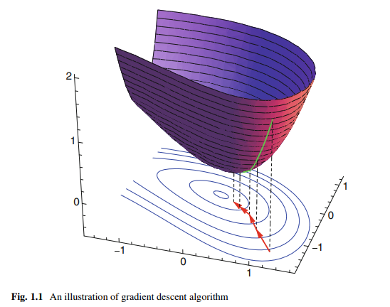
Suppose we start from a point $\boldsymbol{x}_0 \in \mathbb{R}^n$. If the function $f(\boldsymbol{x})$ is defined and differentiable in a neighborhood of $\boldsymbol{x}_0$, then $f(\boldsymbol{x})$ decreases fastest if we move in the direction of the negative gradient of $\nabla f(\boldsymbol{x})$ at $\boldsymbol{x}_0$. When we move a small enough distance, in other words, for a small enough $\gamma_0>0$, we reach a new point $\boldsymbol{x}_1$
$$
\boldsymbol{x}_1=\boldsymbol{x}_0-\gamma_0 \nabla f\left(\boldsymbol{x}_0\right)
$$
and it follows that
$$
f\left(x_0\right) \geq f\left(x_1\right)
$$
Consider the sequence $\left{\boldsymbol{x}0, \boldsymbol{x}_1, \ldots, \boldsymbol{x}_k\right}$ such that $$ \boldsymbol{x}{k+1}=\boldsymbol{x}_k-\gamma_k \nabla f\left(\boldsymbol{x}_k\right), \gamma_k>0
$$
we have
$$
f\left(\boldsymbol{x}0\right) \geq f\left(\boldsymbol{x}_1\right) \geq \cdots f\left(\boldsymbol{x}_k\right) \geq f\left(\boldsymbol{x}{k+1}\right) \geq \cdots
$$
and hopefully this sequence converges to the desired local minimum [9]; see Fig. 1.1 for an illustration.
We call such search algorithm as gradient descent algorithm. When the function $f(\boldsymbol{x})$ is convex, all local minima are meanwhile the global minima, and gradient descent algorithm can converge to the global solution.
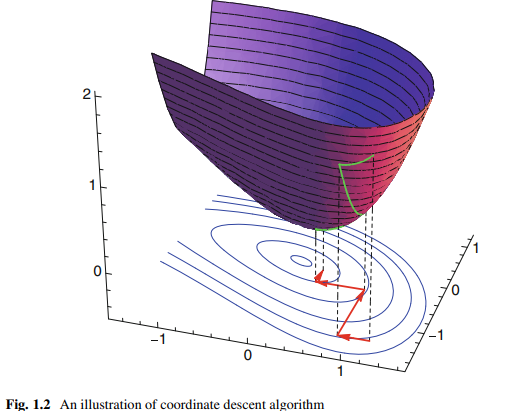
Another widely used search strategy is coordinate descent algorithm. It is based on the fact that the minimization of a multivariate function can be achieved by iteratively minimizing it along one direction at each time [10]. For the above problem (1.17), we can iterate through each direction, one at a time, minimizing the objective function with respect that coordinate direction as
$$
\boldsymbol{x}i^{k+1}=\arg \min {\boldsymbol{y} \in \mathbb{R}} f\left(x_1^{k+1}, \ldots, x_{i-1}^{k+1}, y, x_{i+1}^k, \ldots, x_n^k\right)
$$
This will generate a sequence $\left{\boldsymbol{x}_0, \boldsymbol{x}_1, \ldots, \boldsymbol{x}_k, \ldots\right}$ such that $f\left(\boldsymbol{x}_0\right) \geq f\left(\boldsymbol{x}_1\right) \geq$ $\cdots f\left(x_k\right) \geq \cdots$. If this multivariate function is a convex function, this sequence will finally reach the global optimal solution; see Fig. 1.2 for an illustration.
数学代写|凸优化作业代写Convex Optimization代考|Karush-Kuhn-Tucker (KKT) Conditions
However, when there are constraints for the optimization problems, we cannot move in a direction that only depends on the gradient of objective function. Let us consider the following minimization problem with constraints
$$
\begin{aligned}
& \min _{\boldsymbol{x}} f(\boldsymbol{x}) \
& \text { s.t. } g_i(\boldsymbol{x}) \leq 0, i=1, \ldots, m
\end{aligned}
$$
where the functions $g_i: \mathbb{R}^n \mapsto \mathbb{R}, i=1, \ldots, m$ are the inequality constraint functions. Suppose the domain of this problem is denoted by $\Omega$. A point $x^*$ is called the optimal solution of the optimization problem, if its objective value is the smallest among all vectors satisfying the constraints.
The Lagrangian function associated with the optimization problem (1.25)-(1.26) is defined as
$$
L(\boldsymbol{x}, \boldsymbol{\alpha})=f(\boldsymbol{x})+\sum_{i=1}^m \alpha_i g_i(\boldsymbol{x})
$$
where $\boldsymbol{\alpha}=\left[\alpha_1, \ldots, \alpha_m\right]^T \in \mathbb{R}^{m+}$ is called a dual variable or Lagrange multiplier vector. The scalar $\alpha_i$ is referred to as the Lagrange multiplier associated with the $i$ th constraint.
The Lagrange dual function is defined as the infimum of the Lagrangian function with respect to $\boldsymbol{\alpha}$
$$
q(\boldsymbol{\alpha})=\inf _{\boldsymbol{x} \in \Omega} L(\boldsymbol{x}, \boldsymbol{\alpha})
$$
Denote the optimal value of primal problem (1.25)-(1.26) by $f^$. It can be easily shown that $q(\boldsymbol{\alpha}) \leq f^$. This is called weak duality.
凸优化代写
数学代写|凸优化作业代写Convex Optimization代考|Gradient Descent and Coordinate Descent
让我们考虑一个没有约束的最小化问题
$$
\min _{\boldsymbol{x}} f(\boldsymbol{x})
$$
其中$\boldsymbol{x} \in \mathbb{R}^n$为优化变量,$f: \mathbb{R}^n \mapsto \mathbb{R}$为目标函数。
假设我们从一点$\boldsymbol{x}_0 \in \mathbb{R}^n$开始。如果函数$f(\boldsymbol{x})$被定义并且在$\boldsymbol{x}_0$的邻域内可微,那么如果我们在$\boldsymbol{x}_0$处沿负梯度$\nabla f(\boldsymbol{x})$的方向移动,那么$f(\boldsymbol{x})$减小得最快。当我们移动足够小的距离,换句话说,对于一个足够小的$\gamma_0>0$,我们到达一个新的点 $\boldsymbol{x}_1$
$$
\boldsymbol{x}_1=\boldsymbol{x}_0-\gamma_0 \nabla f\left(\boldsymbol{x}_0\right)
$$
因此
$$
f\left(x_0\right) \geq f\left(x_1\right)
$$
考虑顺序$\left{\boldsymbol{x}0, \boldsymbol{x}_1, \ldots, \boldsymbol{x}_k\right}$,这样$$ \boldsymbol{x}{k+1}=\boldsymbol{x}_k-\gamma_k \nabla f\left(\boldsymbol{x}_k\right), \gamma_k>0
$$
我们有
$$
f\left(\boldsymbol{x}0\right) \geq f\left(\boldsymbol{x}_1\right) \geq \cdots f\left(\boldsymbol{x}_k\right) \geq f\left(\boldsymbol{x}{k+1}\right) \geq \cdots
$$
希望这个序列收敛到期望的局部最小值[9];如图1.1所示。
我们称这种搜索算法为梯度下降算法。当函数$f(\boldsymbol{x})$为凸时,所有的局部极小值同时也是全局极小值,梯度下降算法可以收敛到全局解。
另一种广泛使用的搜索策略是坐标下降算法。它基于这样一个事实,即多元函数的最小化可以通过每次沿一个方向迭代最小化来实现[10]。对于上面的问题(1.17),我们可以在每个方向上迭代,一次一个,使目标函数相对于坐标方向的最小值为
$$
\boldsymbol{x}i^{k+1}=\arg \min {\boldsymbol{y} \in \mathbb{R}} f\left(x_1^{k+1}, \ldots, x_{i-1}^{k+1}, y, x_{i+1}^k, \ldots, x_n^k\right)
$$
这将生成一个序列$\left{\boldsymbol{x}_0, \boldsymbol{x}_1, \ldots, \boldsymbol{x}_k, \ldots\right}$,例如$f\left(\boldsymbol{x}_0\right) \geq f\left(\boldsymbol{x}_1\right) \geq$$\cdots f\left(x_k\right) \geq \cdots$。如果此多元函数为凸函数,则该序列最终将达到全局最优解;如图1.2所示。
数学代写|凸优化作业代写Convex Optimization代考|Karush-Kuhn-Tucker (KKT) Conditions
然而,当优化问题存在约束条件时,我们不能只依赖于目标函数的梯度方向运动。让我们考虑下面这个有约束的最小化问题
$$
\begin{aligned}
& \min _{\boldsymbol{x}} f(\boldsymbol{x}) \
& \text { s.t. } g_i(\boldsymbol{x}) \leq 0, i=1, \ldots, m
\end{aligned}
$$
其中$g_i: \mathbb{R}^n \mapsto \mathbb{R}, i=1, \ldots, m$是不等式约束函数。假设这个问题的定义域用$\Omega$表示。如果点$x^*$的目标值在满足约束的所有向量中最小,则称为优化问题的最优解。
与优化问题(1.25)-(1.26)相关的拉格朗日函数定义为
$$
L(\boldsymbol{x}, \boldsymbol{\alpha})=f(\boldsymbol{x})+\sum_{i=1}^m \alpha_i g_i(\boldsymbol{x})
$$
其中$\boldsymbol{\alpha}=\left[\alpha_1, \ldots, \alpha_m\right]^T \in \mathbb{R}^{m+}$称为对偶变量或拉格朗日乘子向量。标量$\alpha_i$被称为与$i$第1个约束相关联的拉格朗日乘子。
拉格朗日对偶函数定义为拉格朗日函数对$\boldsymbol{\alpha}$的极小值
$$
q(\boldsymbol{\alpha})=\inf _{\boldsymbol{x} \in \Omega} L(\boldsymbol{x}, \boldsymbol{\alpha})
$$
用$f^$表示原始问题(1.25)-(1.26)的最优值。可以很容易地证明$q(\boldsymbol{\alpha}) \leq f^$。这被称为弱对偶。

统计代写请认准statistics-lab™. statistics-lab™为您的留学生涯保驾护航。
微观经济学代写
微观经济学是主流经济学的一个分支,研究个人和企业在做出有关稀缺资源分配的决策时的行为以及这些个人和企业之间的相互作用。my-assignmentexpert™ 为您的留学生涯保驾护航 在数学Mathematics作业代写方面已经树立了自己的口碑, 保证靠谱, 高质且原创的数学Mathematics代写服务。我们的专家在图论代写Graph Theory代写方面经验极为丰富,各种图论代写Graph Theory相关的作业也就用不着 说。
线性代数代写
线性代数是数学的一个分支,涉及线性方程,如:线性图,如:以及它们在向量空间和通过矩阵的表示。线性代数是几乎所有数学领域的核心。
博弈论代写
现代博弈论始于约翰-冯-诺伊曼(John von Neumann)提出的两人零和博弈中的混合策略均衡的观点及其证明。冯-诺依曼的原始证明使用了关于连续映射到紧凑凸集的布劳威尔定点定理,这成为博弈论和数学经济学的标准方法。在他的论文之后,1944年,他与奥斯卡-莫根斯特恩(Oskar Morgenstern)共同撰写了《游戏和经济行为理论》一书,该书考虑了几个参与者的合作游戏。这本书的第二版提供了预期效用的公理理论,使数理统计学家和经济学家能够处理不确定性下的决策。
微积分代写
微积分,最初被称为无穷小微积分或 “无穷小的微积分”,是对连续变化的数学研究,就像几何学是对形状的研究,而代数是对算术运算的概括研究一样。
它有两个主要分支,微分和积分;微分涉及瞬时变化率和曲线的斜率,而积分涉及数量的累积,以及曲线下或曲线之间的面积。这两个分支通过微积分的基本定理相互联系,它们利用了无限序列和无限级数收敛到一个明确定义的极限的基本概念 。
计量经济学代写
什么是计量经济学?
计量经济学是统计学和数学模型的定量应用,使用数据来发展理论或测试经济学中的现有假设,并根据历史数据预测未来趋势。它对现实世界的数据进行统计试验,然后将结果与被测试的理论进行比较和对比。
根据你是对测试现有理论感兴趣,还是对利用现有数据在这些观察的基础上提出新的假设感兴趣,计量经济学可以细分为两大类:理论和应用。那些经常从事这种实践的人通常被称为计量经济学家。
Matlab代写
MATLAB 是一种用于技术计算的高性能语言。它将计算、可视化和编程集成在一个易于使用的环境中,其中问题和解决方案以熟悉的数学符号表示。典型用途包括:数学和计算算法开发建模、仿真和原型制作数据分析、探索和可视化科学和工程图形应用程序开发,包括图形用户界面构建MATLAB 是一个交互式系统,其基本数据元素是一个不需要维度的数组。这使您可以解决许多技术计算问题,尤其是那些具有矩阵和向量公式的问题,而只需用 C 或 Fortran 等标量非交互式语言编写程序所需的时间的一小部分。MATLAB 名称代表矩阵实验室。MATLAB 最初的编写目的是提供对由 LINPACK 和 EISPACK 项目开发的矩阵软件的轻松访问,这两个项目共同代表了矩阵计算软件的最新技术。MATLAB 经过多年的发展,得到了许多用户的投入。在大学环境中,它是数学、工程和科学入门和高级课程的标准教学工具。在工业领域,MATLAB 是高效研究、开发和分析的首选工具。MATLAB 具有一系列称为工具箱的特定于应用程序的解决方案。对于大多数 MATLAB 用户来说非常重要,工具箱允许您学习和应用专业技术。工具箱是 MATLAB 函数(M 文件)的综合集合,可扩展 MATLAB 环境以解决特定类别的问题。可用工具箱的领域包括信号处理、控制系统、神经网络、模糊逻辑、小波、仿真等。