标签: INFS 768

统计代写 | Statistical Learning and Decision Making代考| Inference in Bayesian Networks

如果你也在 怎样代写Statistical Learning and Decision Making这个学科遇到相关的难题,请随时右上角联系我们的24/7代写客服。

数据和预测模型是决策中一个越来越重要的部分。

statistics-lab™ 为您的留学生涯保驾护航 在代写Statistical Learning and Decision Making方面已经树立了自己的口碑, 保证靠谱, 高质且原创的统计Statistics代写服务。我们的专家在代写Statistical Learning and Decision Making代写方面经验极为丰富,各种代写Statistical Learning and Decision Making相关的作业也就用不着说。

我们提供的Statistical Learning and Decision Making及其相关学科的代写,服务范围广, 其中包括但不限于:

  • Statistical Inference 统计推断
  • Statistical Computing 统计计算
  • Advanced Probability Theory 高等楖率论
  • Advanced Mathematical Statistics 高等数理统计学
  • (Generalized) Linear Models 广义线性模型
  • Statistical Machine Learning 统计机器学习
  • Longitudinal Data Analysis 纵向数据分析
  • Foundations of Data Science 数据科学基础
统计代写 | Statistical Learning and Decision Making代考| Inference in Bayesian Networks

统计代写 | Statistical Learning and Decision Making代考|Inference in Bayesian Networks

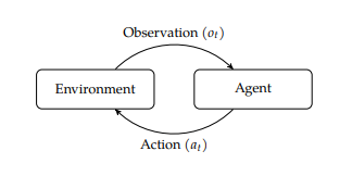
In inference problems, we want to infer a distribution over query variables given some observed evidence variables. The other nodes are referred to as hidden variables. We often refer to the distribution over the query variables given the evidence as a posterior distribution.

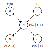
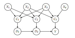
To illustrate the computations involved in inference, recall the Bayesian network from example $2.5$, the structure of which is reproduced in figure $3.1$. Suppose we have $B$ as a query variable and evidence $D=1$ and $C=1$. The inference task is to compute $P\left(b^{1} \mid d^{1}, c^{1}\right)$, which corresponds to computing the probability that we have a battery failure given an observed trajectory deviation and communication loss.

From the definition of conditional probability introduced in equation (2.22), we know
$$
P\left(b^{1} \mid d^{1}, c^{1}\right)=\frac{P\left(b^{1}, d^{1}, c^{1}\right)}{P\left(d^{1}, c^{1}\right)}
$$

To compute the numerator, we must use a process known as marginalization, where we sum out variables that are not involved, in this case $S$ and $E$ :
$$
P\left(b^{1}, d^{1}, c^{1}\right)=\sum_{s} \sum_{e} P\left(b^{1}, s, e, d^{1}, c^{1}\right)
$$
We know from the chain rule for Bayesian networks introduced in equation (2.31) that
$$
P\left(b^{1}, s, e, d^{1}, c^{1}\right)=P\left(b^{1}\right) P(s) P\left(e \mid b^{1}, s\right) P\left(d^{1} \mid e\right) P\left(c^{1} \mid e\right)
$$
All of the components on the right-hand side are specified in the conditional probability distributions associated with the nodes in the Bayesian network. We can compute the denominator in equation (3.1) using the same approach but with anditional summation over the values for $B$.

This process of using the definition of conditional probability, marginalization, and applying the chain rule can be used to perform exact inference in any Bayesian network. We can implement exact inference using factors. Recall that factors represent discrete multivariate distributions. We use the following three operations on factors to achieve this:

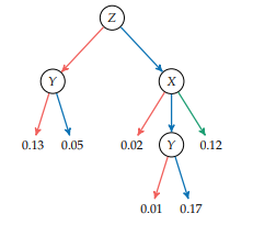
  • We use the factor product (algorithm 3.1) to combine two factors to produce a larger factor whose scope is the combined scope of the input factors. If we have $\phi(X, Y)$ and $\psi(Y, Z)$, then $\phi \cdot \psi$ will be over $X, Y$, and $Z$ with $(\phi \cdot \psi)(x, y, z)=$ $\phi(x, y) \psi(y, z)$. The factor product is demonstrated in example $3.1$.
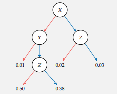
  • We use factor marginalization (algorithm 3.2) to sum out a particular variable from the entire factor table, removing it from the resulting scope. Example $3.2$ illustrates this process.
  • We use factor conditioning (algorithm 3.3) with respect to some evidence to remove any rows in the table inconsistent with that evidence. Example $3 \cdot 3$ demonstrates factor conditioning.

统计代写 | Statistical Learning and Decision Making代考|Inference in Naive Bayes Models

The previous section presented a general method for performing exact inference in any Bayesian network. This section discusses how this same method can be used to solve classification problems for a special kind of Bayesian network structure known as a naive Bayes model. This structure is shown in figure 3.2. An equivalent but more compact representation is shown in figure $3.3$ using a plate, shown as a rounded box. The $i=1: n$ in the bottom of the box specifies that the $i$ in the subscript of the variable name is repeated from 1 to $n$.

In the naive Bayes model, the class $C$ is the query variable, and the observed features $O_{1: n}$ are the evidence variables. The naive Bayes model is called naive because it assumes conditional independence between the evidence variables given the class. Using the notation introduced in section 2.6, we can say $\left(O_{i} \perp O_{j}\right.$ C) for all $i \neq j$. Of course, if these conditional independence assumptions do not hold, then we can add the necessary directed edges between the observed features.

We have to specify the prior $P(C)$ and the class-conditional distributions $P\left(O_{i} \mid C\right)$. As done in the previous section, we can apply the chain rule to compute the joint distribution:
$$
P\left(c, o_{1: n}\right)=P(c) \prod_{i=1}^{n} P\left(o_{i} \mid c\right)
$$
Our classification task involves computing the conditional probability $P\left(c \mid o_{1: n}\right)$. From the definition of conditional probability, we have
$$
P\left(c \mid o_{1: n}\right)=\frac{P\left(c, o_{1: n}\right)}{P\left(o_{1: n}\right)}
$$

We can compute the denominator by marginalizing the joint distribution:
$$
P\left(o_{1: n}\right)=\sum_{c} P\left(c, o_{1: n}\right)
$$
The denominator in equation (3.5) is not a function of $C$ and can therefore be treated as a constant. Hence, we can write
$$
P\left(c \mid o_{1: n}\right)=\kappa P\left(c, o_{1: n}\right)
$$
where $\kappa$ is a normalization constant such that $\sum_{c} P\left(c \mid o_{1: n}\right)=1$. We often drop $\kappa$ and write
$$
P\left(c \mid o_{1: n}\right) \propto P\left(c, o_{1 \Omega}\right)
$$
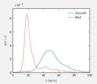
where the proportional to symbol $\propto$ is used to represent that the left-hand side is proportional to the right-hand side. Example $3.4$ illustrates how inference can be applied to classifying radar tracks.

We can use this method to infer a distribution over classes, but for many applications, we have to commit to a particular class. It is common to classify according to the class with the highest posterior probability, $\arg \max {c} P\left(c \mid o{1: n}\right)$. However, choosing a class is really a decision problem that often should take into account the consequences of misclassification. For example, if we are interested in using our classifier to filter out targets that are not aircraft for the purpose of air traffic control, then we can afford to occasionally let a few birds and other clutter tracks through our filter. However, we would want to avoid filtering out any real aircraft because that could lead to a collision. In this case, we would probably only want to classify a track as a bird if the posterior probability were close to $1 .$ Decision problems will be discussed in chapter $6 .$

统计代写 | Statistical Learning and Decision Making代考|Sum-Product Variable Elimination

A variety of methods can be used to perform efficient inference in more complicated Bayesian networks. One method is known as sum-product variable elimination, which interleaves eliminating hidden variables (summations) with applications of the chain rule (products). It is more efficient to marginalize variables out as early as possible to avoid generating large factors.

We will illustrate the variable elimination algorithm by computing the distribution $P\left(B \mid d^{1}, c^{1}\right)$ for the Bayesian network in figure $3.1$. The conditional probability distributions associated with the nodes in the network can be represented by the following factors:
$$
\phi_{1}(B), \phi_{2}(S), \phi_{3}(E, B, S), \phi_{4}(D, E), \phi_{5}(C, E)
$$
Because $D$ and $C$ are observed variables, the last two factors can be replaced with $\phi_{6}(E)$ and $\phi_{7}(E)$ by setting the evidence $D=1$ and $C=1$.

We then proceed by eliminating the hidden variables in sequence. Different strategies can be used for choosing an ordering, but for this example, we arbitrarily choose the ordering $E$ and then $S$. To eliminate $E$, we take the product of all the factors involving $E$ and then marginalize out $E$ to get a new factor:
$$
\phi_{8}(B, S)=\sum_{e} \phi_{3}(e, B, S) \phi_{6}(e) \phi_{7}(e)
$$
We can now discard $\phi_{3}, \phi_{6}$, and $\phi_{7}$ because all the information we need from them is contained in $\phi_{8}$.

Next, we eliminate $S$. Again, we gather all remaining factors that involve $S$ and marginalize out $S$ from the product of these factors:
$$
\phi_{9}(B)=\sum_{s} \phi_{2}(s) \phi_{8}(B, s)
$$
We discard $\phi_{2}$ and $\phi_{8}$, and are left with $\phi_{1}(B)$ and $\phi_{9}(B)$. Finally, we take the product of these two factors and normalize the result to obtain a factor representing $P\left(B \mid d^{1}, c^{1}\right) .$
The above procedure is equivalent to computing the following:
$$
P\left(B \mid d^{1}, c^{1}\right) \propto \phi_{1}(B) \sum_{s}\left(\phi_{2}(s) \sum_{e}\left(\phi_{3}\left(e \mid B_{t} s\right) \phi_{4}\left(d^{1} \mid e\right) \phi_{5}\left(c^{1} \mid e\right)\right)\right)
$$
This produces the same result as, but is more efficient than, the naive procedure of taking the product of all of the factors and then marginalizing:
$$
P\left(B \mid d^{1}, c^{1}\right) \propto \sum_{s} \sum_{e} \phi_{1}(B) \phi_{2}(s) \phi_{3}(e \mid B, s) \phi_{4}\left(d^{1} \mid e\right) \phi_{5}\left(c^{1} \mid e\right)
$$

统计代写 | Statistical Learning and Decision Making代考| Inference in Bayesian Networks

统计代写

统计代写 | Statistical Learning and Decision Making代考|Inference in Bayesian Networks

在推理问题中,我们希望在给定一些观察到的证据变量的情况下推断查询变量的分布。其他节点称为隐藏变量。我们经常将给定证据的查询变量上的分布称为后验分布。

为了说明推理中涉及的计算,请从示例中回顾贝叶斯网络2.5,其结构如图所示3.1. 假设我们有乙作为查询变量和证据D=1和C=1. 推理任务是计算磷(b1∣d1,C1),这对应于在给定观察到的轨迹偏差和通信丢失的情况下计算我们发生电池故障的概率。

由式(2.22)中引入的条件概率的定义,我们知道
磷(b1∣d1,C1)=磷(b1,d1,C1)磷(d1,C1)

为了计算分子,我们必须使用称为边缘化的过程,在这种情况下,我们将不涉及的变量相加小号和和 :
磷(b1,d1,C1)=∑s∑和磷(b1,s,和,d1,C1)
我们从等式(2.31)中引入的贝叶斯网络的链式法则知道
磷(b1,s,和,d1,C1)=磷(b1)磷(s)磷(和∣b1,s)磷(d1∣和)磷(C1∣和)
右侧的所有组件都在与贝叶斯网络中的节点相关的条件概率分布中指定。我们可以使用相同的方法计算等式(3.1)中的分母,但对乙.

这个使用条件概率定义、边缘化和应用链式规则的过程可用于在任何贝叶斯网络中执行精确推理。我们可以使用因子来实现精确推理。回想一下,因子代表离散的多元分布。我们对因子使用以下三个操作来实现这一点:

  • 我们使用因子乘积(算法 3.1)将两个因子组合起来产生一个更大的因子,其范围是输入因子的组合范围。如果我们有φ(X,是)和ψ(是,从), 然后φ⋅ψ将会结束X,是, 和从和(φ⋅ψ)(X,是,和)= φ(X,是)ψ(是,和). 因子积在例子中演示3.1.
  • 我们使用因子边缘化(算法 3.2)从整个因子表中总结出特定变量,将其从结果范围中删除。例子3.2说明了这个过程。
  • 我们针对某些证据使用因子条件(算法 3.3)来删除表中与该证据不一致的任何行。例子3⋅3演示因子调节。

统计代写 | Statistical Learning and Decision Making代考|Inference in Naive Bayes Models

上一节介绍了在任何贝叶斯网络中执行精确推理的通用方法。本节讨论如何使用相同的方法解决一种特殊的贝叶斯网络结构(称为朴素贝叶斯模型)的分类问题。这种结构如图 3.2 所示。等效但更紧凑的表示如图所示3.3使用盘子,显示为圆形框。这一世=1:n在框的底部指定一世在变量名的下标从1到重复n.

在朴素贝叶斯模型中,类C是查询变量,观察到的特征这1:n是证据变量。朴素贝叶斯模型被称为朴素,因为它假设给定类的证据变量之间的条件独立。使用第 2.6 节中介绍的符号,我们可以说(这一世⊥这jC) 为所有人一世≠j. 当然,如果这些条件独立性假设不成立,那么我们可以在观察到的特征之间添加必要的有向边。

我们必须指定先验磷(C)和类条件分布磷(这一世∣C). 如上一节所述,我们可以应用链式法则来计算联合分布:
磷(C,这1:n)=磷(C)∏一世=1n磷(这一世∣C)
我们的分类任务涉及计算条件概率磷(C∣这1:n). 根据条件概率的定义,我们有
磷(C∣这1:n)=磷(C,这1:n)磷(这1:n)

我们可以通过边缘化联合分布来计算分母:
磷(这1:n)=∑C磷(C,这1:n)
等式 (3.5) 中的分母不是C因此可以被视为一个常数。因此,我们可以写
磷(C∣这1:n)=ķ磷(C,这1:n)
在哪里ķ是一个归一化常数,使得∑C磷(C∣这1:n)=1. 我们经常掉线ķ和写
磷(C∣这1:n)∝磷(C,这1Ω)
其中与符号成比例∝用来表示左边与右边成正比。例子3.4说明了如何将推理应用于对雷达轨迹进行分类。

我们可以使用这种方法来推断类的分布,但是对于许多应用程序,我们必须提交到特定的类。通常根据后验概率最高的类别进行分类,参数⁡最大限度C磷(C∣这1:n). 然而,选择一个类别确实是一个决策问题,通常应该考虑错误分类的后果。例如,如果我们有兴趣使用我们的分类器来过滤掉不是飞机的目标以进行空中交通管制,那么我们可以偶尔让一些鸟类和其他杂波轨迹通过我们的过滤器。但是,我们希望避免过滤掉任何真实的飞机,因为这可能会导致碰撞。在这种情况下,如果后验概率接近于1.决策问题将在本章讨论6.

统计代写 | Statistical Learning and Decision Making代考|Sum-Product Variable Elimination

可以使用多种方法在更复杂的贝叶斯网络中执行有效的推理。一种方法称为和积变量消除,它将消除隐藏变量(求和)与链式法则(积)的应用交错。尽早将变量边缘化以避免产生较大的因子更为有效。

我们将通过计算分布来说明变量消除算法磷(乙∣d1,C1)对于图中的贝叶斯网络3.1. 与网络中的节点相关的条件概率分布可以由以下因素表示:
φ1(乙),φ2(小号),φ3(和,乙,小号),φ4(D,和),φ5(C,和)
因为D和C是观察变量,最后两个因子可以替换为φ6(和)和φ7(和)通过设置证据D=1和C=1.

然后我们依次消除隐藏变量。可以使用不同的策略来选择排序,但是对于这个例子,我们任意选择排序和进而小号. 消除和, 我们取所有涉及的因素的乘积和然后边缘化和得到一个新的因素:
φ8(乙,小号)=∑和φ3(和,乙,小号)φ6(和)φ7(和)
我们现在可以丢弃φ3,φ6, 和φ7因为我们需要从他们那里得到的所有信息都包含在φ8.

接下来,我们消除小号. 再次,我们收集了所有涉及的剩余因素小号并边缘化小号从这些因素的产物:
φ9(乙)=∑sφ2(s)φ8(乙,s)
我们丢弃φ2和φ8, 并留下φ1(乙)和φ9(乙). 最后,我们取这两个因子的乘积,并对结果进行归一化,得到一个因子代表磷(乙∣d1,C1).
上述过程等价于计算以下内容:
磷(乙∣d1,C1)∝φ1(乙)∑s(φ2(s)∑和(φ3(和∣乙吨s)φ4(d1∣和)φ5(C1∣和)))
这产生了相同的结果,但比取所有因素的乘积然后边缘化的天真的过程更有效:
磷(乙∣d1,C1)∝∑s∑和φ1(乙)φ2(s)φ3(和∣乙,s)φ4(d1∣和)φ5(C1∣和)

统计代写 | Statistical Learning and Decision Making代考 请认准statistics-lab™

统计代写请认准statistics-lab™. statistics-lab™为您的留学生涯保驾护航。

金融工程代写

金融工程是使用数学技术来解决金融问题。金融工程使用计算机科学、统计学、经济学和应用数学领域的工具和知识来解决当前的金融问题,以及设计新的和创新的金融产品。

非参数统计代写

非参数统计指的是一种统计方法,其中不假设数据来自于由少数参数决定的规定模型;这种模型的例子包括正态分布模型和线性回归模型。

广义线性模型代考

广义线性模型(GLM)归属统计学领域,是一种应用灵活的线性回归模型。该模型允许因变量的偏差分布有除了正态分布之外的其它分布。

术语 广义线性模型(GLM)通常是指给定连续和/或分类预测因素的连续响应变量的常规线性回归模型。它包括多元线性回归,以及方差分析和方差分析(仅含固定效应)。

有限元方法代写

有限元方法(FEM)是一种流行的方法,用于数值解决工程和数学建模中出现的微分方程。典型的问题领域包括结构分析、传热、流体流动、质量运输和电磁势等传统领域。

有限元是一种通用的数值方法,用于解决两个或三个空间变量的偏微分方程(即一些边界值问题)。为了解决一个问题,有限元将一个大系统细分为更小、更简单的部分,称为有限元。这是通过在空间维度上的特定空间离散化来实现的,它是通过构建对象的网格来实现的:用于求解的数值域,它有有限数量的点。边界值问题的有限元方法表述最终导致一个代数方程组。该方法在域上对未知函数进行逼近。[1] 然后将模拟这些有限元的简单方程组合成一个更大的方程系统,以模拟整个问题。然后,有限元通过变化微积分使相关的误差函数最小化来逼近一个解决方案。

tatistics-lab作为专业的留学生服务机构,多年来已为美国、英国、加拿大、澳洲等留学热门地的学生提供专业的学术服务,包括但不限于Essay代写,Assignment代写,Dissertation代写,Report代写,小组作业代写,Proposal代写,Paper代写,Presentation代写,计算机作业代写,论文修改和润色,网课代做,exam代考等等。写作范围涵盖高中,本科,研究生等海外留学全阶段,辐射金融,经济学,会计学,审计学,管理学等全球99%专业科目。写作团队既有专业英语母语作者,也有海外名校硕博留学生,每位写作老师都拥有过硬的语言能力,专业的学科背景和学术写作经验。我们承诺100%原创,100%专业,100%准时,100%满意。

随机分析代写


随机微积分是数学的一个分支,对随机过程进行操作。它允许为随机过程的积分定义一个关于随机过程的一致的积分理论。这个领域是由日本数学家伊藤清在第二次世界大战期间创建并开始的。

时间序列分析代写

随机过程,是依赖于参数的一组随机变量的全体,参数通常是时间。 随机变量是随机现象的数量表现,其时间序列是一组按照时间发生先后顺序进行排列的数据点序列。通常一组时间序列的时间间隔为一恒定值(如1秒,5分钟,12小时,7天,1年),因此时间序列可以作为离散时间数据进行分析处理。研究时间序列数据的意义在于现实中,往往需要研究某个事物其随时间发展变化的规律。这就需要通过研究该事物过去发展的历史记录,以得到其自身发展的规律。

回归分析代写

多元回归分析渐进(Multiple Regression Analysis Asymptotics)属于计量经济学领域,主要是一种数学上的统计分析方法,可以分析复杂情况下各影响因素的数学关系,在自然科学、社会和经济学等多个领域内应用广泛。

MATLAB代写

MATLAB 是一种用于技术计算的高性能语言。它将计算、可视化和编程集成在一个易于使用的环境中,其中问题和解决方案以熟悉的数学符号表示。典型用途包括:数学和计算算法开发建模、仿真和原型制作数据分析、探索和可视化科学和工程图形应用程序开发,包括图形用户界面构建MATLAB 是一个交互式系统,其基本数据元素是一个不需要维度的数组。这使您可以解决许多技术计算问题,尤其是那些具有矩阵和向量公式的问题,而只需用 C 或 Fortran 等标量非交互式语言编写程序所需的时间的一小部分。MATLAB 名称代表矩阵实验室。MATLAB 最初的编写目的是提供对由 LINPACK 和 EISPACK 项目开发的矩阵软件的轻松访问,这两个项目共同代表了矩阵计算软件的最新技术。MATLAB 经过多年的发展,得到了许多用户的投入。在大学环境中,它是数学、工程和科学入门和高级课程的标准教学工具。在工业领域,MATLAB 是高效研究、开发和分析的首选工具。MATLAB 具有一系列称为工具箱的特定于应用程序的解决方案。对于大多数 MATLAB 用户来说非常重要,工具箱允许您学习应用专业技术。工具箱是 MATLAB 函数(M 文件)的综合集合,可扩展 MATLAB 环境以解决特定类别的问题。可用工具箱的领域包括信号处理、控制系统、神经网络、模糊逻辑、小波、仿真等。

R语言代写问卷设计与分析代写
PYTHON代写回归分析与线性模型代写
MATLAB代写方差分析与试验设计代写
STATA代写机器学习/统计学习代写
SPSS代写计量经济学代写
EVIEWS代写时间序列分析代写
EXCEL代写深度学习代写
SQL代写各种数据建模与可视化代写

统计代写 | Statistical Learning and Decision Making代考| Conditional Independence

如果你也在 怎样代写Statistical Learning and Decision Making这个学科遇到相关的难题,请随时右上角联系我们的24/7代写客服。

数据和预测模型是决策中一个越来越重要的部分。

statistics-lab™ 为您的留学生涯保驾护航 在代写Statistical Learning and Decision Making方面已经树立了自己的口碑, 保证靠谱, 高质且原创的统计Statistics代写服务。我们的专家在代写Statistical Learning and Decision Making代写方面经验极为丰富,各种代写Statistical Learning and Decision Making相关的作业也就用不着说。

我们提供的Statistical Learning and Decision Making及其相关学科的代写,服务范围广, 其中包括但不限于:

  • Statistical Inference 统计推断
  • Statistical Computing 统计计算
  • Advanced Probability Theory 高等楖率论
  • Advanced Mathematical Statistics 高等数理统计学
  • (Generalized) Linear Models 广义线性模型
  • Statistical Machine Learning 统计机器学习
  • Longitudinal Data Analysis 纵向数据分析
  • Foundations of Data Science 数据科学基础
统计代写 | Statistical Learning and Decision Making代考| Conditional Independence

统计代写 | Statistical Learning and Decision Making代考|Conditional Independence

The reason that a Bayesian network can represent a joint distribution with fewer independent parameters than would normally be required is due to the conditional independence assumptions encoded in its graphical structure. ${ }^{17}$ Conditional independence is a generalization of the notion of independence introduced in section 2.3-1. Variables $X$ and $Y$ are conditionally independent given $Z$ if and only if $P(X, Y \mid Z)=P(X \mid Z) P(Y \mid Z)$. The assertion that $X$ and $Y$ are conditionally independent given $Z$ is written $(X \perp Y \mid Z$ ). It is possible to show from this definition that $(X \perp Y \mid Z)$ if and only if $P(X \mid Z)=P(X \mid Y, Z)$. Given $Z$, information about $Y$ provides no additional information about $X$, and vice versa. Example $2.6$ provides an example.

We can use a set of rules to determine whether the structure of a Bayesian network implies that two variables must be conditionally independent given a set of other evidence variables. ${ }^{18}$ Suppose we want to check whether $(A \perp B \mid \mathcal{C})$ is implied by the network structure, where $\mathcal{C}$ is a set of evidence variables. We have

to check all possible undirected paths from $A$ to $B$ for what is called $d$-separation. A path between $A$ and $B$ is d-separated by $\mathcal{C}$ if any of the following are true:

  1. The path contains a chain of nodes, $X \rightarrow Y \rightarrow Z$, such that $Y$ is in $\mathcal{C}$.
  2. The path contains a fork, $X \leftarrow Y \rightarrow Z$, such that $Y$ is in $\mathcal{C}$.
  3. The path contains an inverted fork (also called a $v$-structure), $X \rightarrow Y \leftarrow Z$, such that $Y$ is not in $\mathcal{C}$ and no descendant of $Y$ is in $\mathcal{C}$. Example $2.7$ provides some intuition for this rule.

We say that $A$ and $B$ are d-separated by $\mathcal{C}$ if all paths between $A$ and $B$ are $\mathrm{d}-$ separated by $\mathcal{C}$. This d-separation implies that $(A \perp B \mid \mathcal{C}) .{ }^{19}$ Example $2.8$ demonstrates this process for checking whether a graph implies a particular conditional independence assumption.

Sometimes the term Markoo blanket ${ }^{20}$ of a node $X$ is used to refer to the minimal set of nodes that, if their values were known, makes $X$ conditionally independent of all other nodes. A Markov blanket of a particular node turns out to consist of its parents, its children, and the other parents of its children.

统计代写 | Statistical Learning and Decision Making代考|Summary

Representing uncertainty as a probability distribution is motivated by a set of axioms related to the comparison of the plausibility of different statements.
There are many different families of both discrete and continuous probability distributions.Continuous probability distributions can be represented by density functions.

Probability distribution families can be combined together in mixtures to result in more flexible distributions.

Joint distributions are distributions over multiple variables.

Conditional distributions are distributions over one or more variables given values of evidence variables.

A Bayesian network is defined by a graphical structure and a set of conditional distributions.

Depending on the structure of the Bayesian network, we can represent joint distributions with fewer parameters due to conditional independence assumptions.

统计代写 | Statistical Learning and Decision Making代考|Exercises

Exercise 2.1. Consider a continuous random variable $X$ that follows the exponential distribution parameterized by $\lambda$ with density $p(x \mid \lambda)=\lambda \exp (-\lambda x)$ with nonnegative support. Compute the cumulative distribution function of $X$.

Solution: We start with the definition of the cumulative distribution function. Since the support of the distribution is lower-bounded by $x=0$, there is no probability mass in the interval $(-\infty, 0)$, allowing us to adjust the lower bound of the integral to 0 . After computing the integral, wẻ obtain cdf $X(x)$ :
$$
\begin{aligned}
&\operatorname{cdf}{X}(x)=\int{-\infty}^{x} p\left(x^{\prime}\right) \mathrm{d} x^{\prime} \
&\operatorname{cdf}{X}(x)=\int{0}^{x} \lambda e^{-\lambda x^{\prime}} \mathrm{d} x^{\prime} \
&\operatorname{cdf}{X}(x)=-\left.e^{-\lambda x^{\prime}}\right|{0} ^{x} \
&\operatorname{cdf}_{X}(x)=1-e^{-\lambda x}
\end{aligned}
$$
Exercise 2.2. For the density function in figure 2.6, what are the five components of the mixture? (There are multiple valid solutions.)

Solution: One solution is $\mathcal{U}([-10,-10],[-5,10]), \mathcal{U}([-5,0],[0,10]), \mathcal{U}([-5,-10],[0,0])$, $\mathcal{U}([0,-10],[10,5])$, and $\mathcal{U}([0,5],[10,10])$.

Exercise 2.3. Given the following table representation of $P(X, Y, Z)$, generate an equivalent compact decision tree representation.

统计代写 | Statistical Learning and Decision Making代考| Conditional Independence

统计代写

统计代写 | Statistical Learning and Decision Making代考|Conditional Independence

贝叶斯网络可以用比通常需要的更少的独立参数表示联合分布的原因是由于其图形结构中编码的条件独立性假设。17条件独立是对 2.3-1 节中引入的独立概念的概括。变量X和是是有条件独立给定的从当且仅当磷(X,是∣从)=磷(X∣从)磷(是∣从). 断言X和是是有条件独立给定的从写着(X⊥是∣从)。从这个定义可以证明(X⊥是∣从)当且仅当磷(X∣从)=磷(X∣是,从). 给定从, 相关信息是没有提供关于X,反之亦然。例子2.6提供了一个例子。

我们可以使用一组规则来确定贝叶斯网络的结构是否意味着在给定一组其他证据变量的情况下两个变量必须条件独立。18假设我们要检查是否(一种⊥乙∣C)由网络结构隐含,其中C是一组证据变量。我们有

检查所有可能的无向路径一种到乙对于所谓的d-分离。之间的路径一种和乙由 d 分隔C如果以下任何一项为真:

  1. 路径包含一系列节点,X→是→从, 这样是在C.
  2. 路径包含一个叉子,X←是→从, 这样是在C.
  3. 该路径包含一个倒叉(也称为在-结构体),X→是←从, 这样是不在C并且没有后代是在C. 例子2.7为这条规则提供了一些直觉。

我们说一种和乙由 d 分隔C如果之间的所有路径一种和乙是d−由C. 这种 d-分离意味着(一种⊥乙∣C).19例子2.8演示了检查图是否暗示特定条件独立性假设的过程。

有时术语 Markoo 毯子20一个节点的X用于指代最小的节点集,如果它们的值已知,则使X有条件地独立于所有其他节点。一个特定节点的马尔可夫毯最终由它的父母、它的孩子和它的孩子的其他父母组成。

统计代写 | Statistical Learning and Decision Making代考|Summary

将不确定性表示为概率分布是由一组与比较不同陈述的合理性相关的公理推动的。
离散和连续概率分布有许多不同的族。连续概率分布可以用密度函数表示。

概率分布族可以混合在一起,以产生更灵活的分布。

联合分布是多个变量的分布。

条件分布是给定证据变量值的一个或多个变量的分布。

贝叶斯网络由图形结构和一组条件分布定义。

根据贝叶斯网络的结构,由于条件独立假设,我们可以用更少的参数表示联合分布。

统计代写 | Statistical Learning and Decision Making代考|Exercises

练习 2.1。考虑一个连续随机变量X遵循参数化的指数分布λ有密度p(X∣λ)=λ经验⁡(−λX)在非负支持下。计算累积分布函数X.

解:我们从累积分布函数的定义开始。由于分布的支持下界为X=0,区间内没有概率质量(−∞,0),允许我们将积分的下限调整为 0 。计算积分后,wẻ得到cdfX(X) :
cdf⁡X(X)=∫−∞Xp(X′)dX′ cdf⁡X(X)=∫0Xλ和−λX′dX′ cdf⁡X(X)=−和−λX′|0X cdfX⁡(X)=1−和−λX
练习 2.2。对于图 2.6 中的密度函数,混合物的五种成分是什么?(有多种有效的解决方案。)

解决方案:一种解决方案是在([−10,−10],[−5,10]),在([−5,0],[0,10]),在([−5,−10],[0,0]), 在([0,−10],[10,5]), 和在([0,5],[10,10]).

练习 2.3。给定下表表示磷(X,是,从),生成等效的紧凑决策树表示。

统计代写 | Statistical Learning and Decision Making代考 请认准statistics-lab™

统计代写请认准statistics-lab™. statistics-lab™为您的留学生涯保驾护航。

金融工程代写

金融工程是使用数学技术来解决金融问题。金融工程使用计算机科学、统计学、经济学和应用数学领域的工具和知识来解决当前的金融问题,以及设计新的和创新的金融产品。

非参数统计代写

非参数统计指的是一种统计方法,其中不假设数据来自于由少数参数决定的规定模型;这种模型的例子包括正态分布模型和线性回归模型。

广义线性模型代考

广义线性模型(GLM)归属统计学领域,是一种应用灵活的线性回归模型。该模型允许因变量的偏差分布有除了正态分布之外的其它分布。

术语 广义线性模型(GLM)通常是指给定连续和/或分类预测因素的连续响应变量的常规线性回归模型。它包括多元线性回归,以及方差分析和方差分析(仅含固定效应)。

有限元方法代写

有限元方法(FEM)是一种流行的方法,用于数值解决工程和数学建模中出现的微分方程。典型的问题领域包括结构分析、传热、流体流动、质量运输和电磁势等传统领域。

有限元是一种通用的数值方法,用于解决两个或三个空间变量的偏微分方程(即一些边界值问题)。为了解决一个问题,有限元将一个大系统细分为更小、更简单的部分,称为有限元。这是通过在空间维度上的特定空间离散化来实现的,它是通过构建对象的网格来实现的:用于求解的数值域,它有有限数量的点。边界值问题的有限元方法表述最终导致一个代数方程组。该方法在域上对未知函数进行逼近。[1] 然后将模拟这些有限元的简单方程组合成一个更大的方程系统,以模拟整个问题。然后,有限元通过变化微积分使相关的误差函数最小化来逼近一个解决方案。

tatistics-lab作为专业的留学生服务机构,多年来已为美国、英国、加拿大、澳洲等留学热门地的学生提供专业的学术服务,包括但不限于Essay代写,Assignment代写,Dissertation代写,Report代写,小组作业代写,Proposal代写,Paper代写,Presentation代写,计算机作业代写,论文修改和润色,网课代做,exam代考等等。写作范围涵盖高中,本科,研究生等海外留学全阶段,辐射金融,经济学,会计学,审计学,管理学等全球99%专业科目。写作团队既有专业英语母语作者,也有海外名校硕博留学生,每位写作老师都拥有过硬的语言能力,专业的学科背景和学术写作经验。我们承诺100%原创,100%专业,100%准时,100%满意。

随机分析代写


随机微积分是数学的一个分支,对随机过程进行操作。它允许为随机过程的积分定义一个关于随机过程的一致的积分理论。这个领域是由日本数学家伊藤清在第二次世界大战期间创建并开始的。

时间序列分析代写

随机过程,是依赖于参数的一组随机变量的全体,参数通常是时间。 随机变量是随机现象的数量表现,其时间序列是一组按照时间发生先后顺序进行排列的数据点序列。通常一组时间序列的时间间隔为一恒定值(如1秒,5分钟,12小时,7天,1年),因此时间序列可以作为离散时间数据进行分析处理。研究时间序列数据的意义在于现实中,往往需要研究某个事物其随时间发展变化的规律。这就需要通过研究该事物过去发展的历史记录,以得到其自身发展的规律。

回归分析代写

多元回归分析渐进(Multiple Regression Analysis Asymptotics)属于计量经济学领域,主要是一种数学上的统计分析方法,可以分析复杂情况下各影响因素的数学关系,在自然科学、社会和经济学等多个领域内应用广泛。

MATLAB代写

MATLAB 是一种用于技术计算的高性能语言。它将计算、可视化和编程集成在一个易于使用的环境中,其中问题和解决方案以熟悉的数学符号表示。典型用途包括:数学和计算算法开发建模、仿真和原型制作数据分析、探索和可视化科学和工程图形应用程序开发,包括图形用户界面构建MATLAB 是一个交互式系统,其基本数据元素是一个不需要维度的数组。这使您可以解决许多技术计算问题,尤其是那些具有矩阵和向量公式的问题,而只需用 C 或 Fortran 等标量非交互式语言编写程序所需的时间的一小部分。MATLAB 名称代表矩阵实验室。MATLAB 最初的编写目的是提供对由 LINPACK 和 EISPACK 项目开发的矩阵软件的轻松访问,这两个项目共同代表了矩阵计算软件的最新技术。MATLAB 经过多年的发展,得到了许多用户的投入。在大学环境中,它是数学、工程和科学入门和高级课程的标准教学工具。在工业领域,MATLAB 是高效研究、开发和分析的首选工具。MATLAB 具有一系列称为工具箱的特定于应用程序的解决方案。对于大多数 MATLAB 用户来说非常重要,工具箱允许您学习应用专业技术。工具箱是 MATLAB 函数(M 文件)的综合集合,可扩展 MATLAB 环境以解决特定类别的问题。可用工具箱的领域包括信号处理、控制系统、神经网络、模糊逻辑、小波、仿真等。

R语言代写问卷设计与分析代写
PYTHON代写回归分析与线性模型代写
MATLAB代写方差分析与试验设计代写
STATA代写机器学习/统计学习代写
SPSS代写计量经济学代写
EVIEWS代写时间序列分析代写
EXCEL代写深度学习代写
SQL代写各种数据建模与可视化代写

统计代写 | Statistical Learning and Decision Making代考|Conditional Distributions

如果你也在 怎样代写Statistical Learning and Decision Making这个学科遇到相关的难题,请随时右上角联系我们的24/7代写客服。

数据和预测模型是决策中一个越来越重要的部分。

statistics-lab™ 为您的留学生涯保驾护航 在代写Statistical Learning and Decision Making方面已经树立了自己的口碑, 保证靠谱, 高质且原创的统计Statistics代写服务。我们的专家在代写Statistical Learning and Decision Making代写方面经验极为丰富,各种代写Statistical Learning and Decision Making相关的作业也就用不着说。

我们提供的Statistical Learning and Decision Making及其相关学科的代写,服务范围广, 其中包括但不限于:

  • Statistical Inference 统计推断
  • Statistical Computing 统计计算
  • Advanced Probability Theory 高等楖率论
  • Advanced Mathematical Statistics 高等数理统计学
  • (Generalized) Linear Models 广义线性模型
  • Statistical Machine Learning 统计机器学习
  • Longitudinal Data Analysis 纵向数据分析
  • Foundations of Data Science 数据科学基础
统计代写 | Statistical Learning and Decision Making代考|Conditional Distributions

统计代写 | Statistical Learning and Decision Making代考|Conditional Distributions

The previous section introduced the idea of independence, which can help reduce the number of parameters used to define a joint distribution. However, as was mentioned, independence can be too strong of an assumption. This section will introduce the idea of conditional independence, which can help reduce the number of independent parameters without making assumptions that are as strong. Before discussing conditional independence, we will first introduce the notion of a conditional distribution, which is a distribution over a variable given the value of one or more others.

The definition of conditional probability states that
$$
P(x \mid y)=\frac{P(x, y)}{P(y)}
$$
where $P(x \mid y)$ is read as “probability of $x$ given $y$.” In some contexts, it is common to refer to $y$ as evidence.

Since a conditional probability distribution is a probability distribution over one or more variables given some evidence, we know that
$$
\sum_{x} P(x \mid y)=1
$$
for a discrete $X$. If $X$ is continuous, it integrates to 1 .
We can incorporate the definition of conditional probability into equation (2.18) to obtain a slightly different form of the law of total probability:
$$
P(x)=\sum_{y} P(x \mid y) P(y)
$$
for a discrete distribution.
Another useful relationship that follows from the definition of conditional probability is Bayes’ rule: ${ }^{12}$
$$
P(x \mid y)=\frac{P(y \mid x) P(x)}{P(y)}
$$
If we have a representation of a conditional distribution $P(y \mid x)$, we can apply Bayes’s rule to swap the $y$ and $x$ to obtain the conditional distribution $P(x \mid y)$.
We will now discuss a variety of ways to represent conditional probability distributions over discrete and continuous variables.

统计代写 | Statistical Learning and Decision Making代考|Discrete Conditional Models

A conditional probability distribution over discrete variables can be represented using a table. In fact, we can use the same discrete factor representation that we used in section $2.3 .1$ for joint distributions. Table $2.3$ shows an example of a table representing $P(X \mid Y, Z)$ with all binary variables. In contrast with a joint table (e.g, table $2.1$ ), the column containing the probabilities need not sum to 1. However, if we sum over the probabilities that are consistent with what we are conditioning on, we must get 1 . For example, conditioning on $y^{0}$ and $z^{0}$ (the evidence), we have
$$
P\left(x^{0} \mid y^{0}, z^{0}\right)+P\left(x^{1} \mid y^{0}, z^{0}\right)=0.08+0.92=1
$$ Conditional probability tables can become quite large. If we were to create a table like table $2.3$ where all variables can take on $m$ values and we are conditioning on $n$ variables, there would be $m^{n+1}$ rows. However, since the $m$ values of the variable we are not conditioning on must sum to 1 , there are only $(m-1) m^{n}$ independent parameters. There is still an exponential growth in the number of variables on which we condition. When there are many repeated values in the conditional probability table, a decision tree (introduced in section 2.3.1) may be a more efficient representation.

统计代写 | Statistical Learning and Decision Making代考|Conditional Linear Gaussian Models

The conditional linear Gaussian model combines the ideas of conditional Gaussian and linear Gaussian models to be able to handle conditioning a continuous variable on both discrete and continuous variables. Suppose we want to represent $p(X \mid Y, Z)$, where $X$ and $Y$ are continuous and $Z$ is discrete with values $1: n$. The conditional density function is then
$$
p(x \mid y, z)= \begin{cases}\mathcal{N}\left(x \mid m_{1} y+b_{1}, \sigma_{1}^{2}\right) & \text { if } z^{1} \ \vdots \ \mathcal{N}\left(x \mid m_{n} y+b_{n}, \sigma_{n}^{2}\right) & \text { if } z^{n}\end{cases}
$$
Above, the parameter vector $\theta=\left[m_{1: n}, b_{1: n}, \sigma_{1: n}\right]$ has $3 n$ components.

We can use a sigmoid ${ }^{13}$ model to represent a distribution over a binary variable conditioned on a continuous variable. For example, we may want to represent $P\left(x^{1} \mid y\right)$, where $x$ is binary and $y$ is continuous. Of course, we could just set a threshold $\theta$ and say $P\left(x^{1} \mid y\right)=0$ if $y<\theta$ and $P\left(x^{1} \mid y\right)=1$ otherwise. However, in many applications, we may not want to have such a hard threshold that results in assigning zero probability to $x^{1}$ for certain values of $y$.

Instead of a hard threshold, we could use a soft threshold that assigns low probabilities when below a threshold and high probabilities when above a threshold. One way to represent a soft threshold is to use a logit model, which produces a sigmoid curve:
$$
P\left(x^{1} \mid y\right)=\frac{1}{1+\exp \left(-2 \frac{y-\theta_{1}}{\theta_{2}}\right)}
$$
The parameter $\theta_{1}$ governs the location of the threshold, and $\theta_{2}$ controls the “softness” or spread of the probabilities. Figure $2.10$ shows an example plot of $P\left(x^{1} \mid y\right)$ with a logit model.

统计代写 | Statistical Learning and Decision Making代考|Conditional Distributions

统计代写

统计代写 | Statistical Learning and Decision Making代考|Conditional Distributions

上一节介绍了独立性的概念,它可以帮助减少用于定义联合分布的参数数量。然而,如前所述,独立性可能过于强大的假设。本节将介绍条件独立的概念,它可以帮助减少独立参数的数量,而无需做出那么强的假设。在讨论条件独立性之前,我们将首先介绍条件分布的概念,它是给定一个或多个其他变量值的变量上的分布。

条件概率的定义表明
磷(X∣是)=磷(X,是)磷(是)
在哪里磷(X∣是)读作“概率X给定是。” 在某些情况下,通常指的是是作为证据。

由于条件概率分布是给定一些证据的一个或多个变量的概率分布,我们知道
∑X磷(X∣是)=1
对于离散X. 如果X是连续的,它积分为 1 。
我们可以将条件概率的定义并入方程(2.18)中,得到一种稍微不同形式的全概率定律:
磷(X)=∑是磷(X∣是)磷(是)
对于离散分布。
从条件概率的定义中得出的另一个有用的关系是贝叶斯规则:12
磷(X∣是)=磷(是∣X)磷(X)磷(是)
如果我们有一个条件分布的表示磷(是∣X),我们可以应用贝叶斯规则来交换是和X获得条件分布磷(X∣是).
我们现在将讨论各种表示离散和连续变量的条件概率分布的方法。

统计代写 | Statistical Learning and Decision Making代考|Discrete Conditional Models

离散变量的条件概率分布可以使用表格来表示。事实上,我们可以使用我们在章节中使用的相同的离散因子表示2.3.1用于联合分布。桌子2.3显示了一个表格示例磷(X∣是,从)与所有二进制变量。与联合表(例如,表2.1),包含概率的列不必总和为 1。但是,如果我们对与我们所依据的条件一致的概率求和,我们必须得到 1。例如,调节是0和和0(证据),我们有
磷(X0∣是0,和0)+磷(X1∣是0,和0)=0.08+0.92=1条件概率表可以变得非常大。如果我们要创建一个类似表的表2.3所有变量都可以承担的地方米价值观,我们正在调整n变量,会有米n+1行。然而,由于米我们不作为条件的变量的值必须总和为 1 ,只有(米−1)米n独立参数。我们所依赖的变量数量仍然呈指数增长。当条件概率表中有很多重复值时,决策树(在 2.3.1 节中介绍)可能是更有效的表示。

统计代写 | Statistical Learning and Decision Making代考|Conditional Linear Gaussian Models

条件线性高斯模型结合了条件高斯和线性高斯模型的思想,能够处理对离散变量和连续变量的连续变量进行调节。假设我们要表示p(X∣是,从), 在哪里X和是是连续的并且从是离散的值1:n. 条件密度函数为
p(X∣是,和)={ñ(X∣米1是+b1,σ12) 如果 和1 ⋮ ñ(X∣米n是+bn,σn2) 如果 和n
上图,参数向量θ=[米1:n,b1:n,σ1:n]拥有3n组件。

我们可以使用 sigmoid13模型来表示以连续变量为条件的二元变量上的分布。例如,我们可能想要表示磷(X1∣是), 在哪里X是二进制的并且是是连续的。当然,我们可以设置一个阈值θ说磷(X1∣是)=0如果是<θ和磷(X1∣是)=1除此以外。然而,在许多应用程序中,我们可能不希望有这样一个硬阈值,导致将零概率分配给X1对于某些值是.

代替硬阈值,我们可以使用软阈值,在低于阈值时分配低概率,在高于阈值时分配高概率。表示软阈值的一种方法是使用 logit 模型,该模型会生成 sigmoid 曲线:
磷(X1∣是)=11+经验⁡(−2是−θ1θ2)
参数θ1控制阈值的位置,并且θ2控制概率的“柔软性”或传播。数字2.10显示了一个示例图磷(X1∣是)使用 logit 模型。

统计代写 | Statistical Learning and Decision Making代考 请认准statistics-lab™

统计代写请认准statistics-lab™. statistics-lab™为您的留学生涯保驾护航。

金融工程代写

金融工程是使用数学技术来解决金融问题。金融工程使用计算机科学、统计学、经济学和应用数学领域的工具和知识来解决当前的金融问题,以及设计新的和创新的金融产品。

非参数统计代写

非参数统计指的是一种统计方法,其中不假设数据来自于由少数参数决定的规定模型;这种模型的例子包括正态分布模型和线性回归模型。

广义线性模型代考

广义线性模型(GLM)归属统计学领域,是一种应用灵活的线性回归模型。该模型允许因变量的偏差分布有除了正态分布之外的其它分布。

术语 广义线性模型(GLM)通常是指给定连续和/或分类预测因素的连续响应变量的常规线性回归模型。它包括多元线性回归,以及方差分析和方差分析(仅含固定效应)。

有限元方法代写

有限元方法(FEM)是一种流行的方法,用于数值解决工程和数学建模中出现的微分方程。典型的问题领域包括结构分析、传热、流体流动、质量运输和电磁势等传统领域。

有限元是一种通用的数值方法,用于解决两个或三个空间变量的偏微分方程(即一些边界值问题)。为了解决一个问题,有限元将一个大系统细分为更小、更简单的部分,称为有限元。这是通过在空间维度上的特定空间离散化来实现的,它是通过构建对象的网格来实现的:用于求解的数值域,它有有限数量的点。边界值问题的有限元方法表述最终导致一个代数方程组。该方法在域上对未知函数进行逼近。[1] 然后将模拟这些有限元的简单方程组合成一个更大的方程系统,以模拟整个问题。然后,有限元通过变化微积分使相关的误差函数最小化来逼近一个解决方案。

tatistics-lab作为专业的留学生服务机构,多年来已为美国、英国、加拿大、澳洲等留学热门地的学生提供专业的学术服务,包括但不限于Essay代写,Assignment代写,Dissertation代写,Report代写,小组作业代写,Proposal代写,Paper代写,Presentation代写,计算机作业代写,论文修改和润色,网课代做,exam代考等等。写作范围涵盖高中,本科,研究生等海外留学全阶段,辐射金融,经济学,会计学,审计学,管理学等全球99%专业科目。写作团队既有专业英语母语作者,也有海外名校硕博留学生,每位写作老师都拥有过硬的语言能力,专业的学科背景和学术写作经验。我们承诺100%原创,100%专业,100%准时,100%满意。

随机分析代写


随机微积分是数学的一个分支,对随机过程进行操作。它允许为随机过程的积分定义一个关于随机过程的一致的积分理论。这个领域是由日本数学家伊藤清在第二次世界大战期间创建并开始的。

时间序列分析代写

随机过程,是依赖于参数的一组随机变量的全体,参数通常是时间。 随机变量是随机现象的数量表现,其时间序列是一组按照时间发生先后顺序进行排列的数据点序列。通常一组时间序列的时间间隔为一恒定值(如1秒,5分钟,12小时,7天,1年),因此时间序列可以作为离散时间数据进行分析处理。研究时间序列数据的意义在于现实中,往往需要研究某个事物其随时间发展变化的规律。这就需要通过研究该事物过去发展的历史记录,以得到其自身发展的规律。

回归分析代写

多元回归分析渐进(Multiple Regression Analysis Asymptotics)属于计量经济学领域,主要是一种数学上的统计分析方法,可以分析复杂情况下各影响因素的数学关系,在自然科学、社会和经济学等多个领域内应用广泛。

MATLAB代写

MATLAB 是一种用于技术计算的高性能语言。它将计算、可视化和编程集成在一个易于使用的环境中,其中问题和解决方案以熟悉的数学符号表示。典型用途包括:数学和计算算法开发建模、仿真和原型制作数据分析、探索和可视化科学和工程图形应用程序开发,包括图形用户界面构建MATLAB 是一个交互式系统,其基本数据元素是一个不需要维度的数组。这使您可以解决许多技术计算问题,尤其是那些具有矩阵和向量公式的问题,而只需用 C 或 Fortran 等标量非交互式语言编写程序所需的时间的一小部分。MATLAB 名称代表矩阵实验室。MATLAB 最初的编写目的是提供对由 LINPACK 和 EISPACK 项目开发的矩阵软件的轻松访问,这两个项目共同代表了矩阵计算软件的最新技术。MATLAB 经过多年的发展,得到了许多用户的投入。在大学环境中,它是数学、工程和科学入门和高级课程的标准教学工具。在工业领域,MATLAB 是高效研究、开发和分析的首选工具。MATLAB 具有一系列称为工具箱的特定于应用程序的解决方案。对于大多数 MATLAB 用户来说非常重要,工具箱允许您学习应用专业技术。工具箱是 MATLAB 函数(M 文件)的综合集合,可扩展 MATLAB 环境以解决特定类别的问题。可用工具箱的领域包括信号处理、控制系统、神经网络、模糊逻辑、小波、仿真等。

R语言代写问卷设计与分析代写
PYTHON代写回归分析与线性模型代写
MATLAB代写方差分析与试验设计代写
STATA代写机器学习/统计学习代写
SPSS代写计量经济学代写
EVIEWS代写时间序列分析代写
EXCEL代写深度学习代写
SQL代写各种数据建模与可视化代写

统计代写 | Statistical Learning and Decision Making代考|Joint Distributions

如果你也在 怎样代写Statistical Learning and Decision Making这个学科遇到相关的难题,请随时右上角联系我们的24/7代写客服。

数据和预测模型是决策中一个越来越重要的部分。

statistics-lab™ 为您的留学生涯保驾护航 在代写Statistical Learning and Decision Making方面已经树立了自己的口碑, 保证靠谱, 高质且原创的统计Statistics代写服务。我们的专家在代写Statistical Learning and Decision Making代写方面经验极为丰富,各种代写Statistical Learning and Decision Making相关的作业也就用不着说。

我们提供的Statistical Learning and Decision Making及其相关学科的代写,服务范围广, 其中包括但不限于:

  • Statistical Inference 统计推断
  • Statistical Computing 统计计算
  • Advanced Probability Theory 高等楖率论
  • Advanced Mathematical Statistics 高等数理统计学
  • (Generalized) Linear Models 广义线性模型
  • Statistical Machine Learning 统计机器学习
  • Longitudinal Data Analysis 纵向数据分析
  • Foundations of Data Science 数据科学基础
统计代写 | Statistical Learning and Decision Making代考|Joint Distributions

统计代写 | Statistical Learning and Decision Making代考|Joint Distributions

A joint distribution is a probability distribution over multiple variables. A distribution over a single variable is called a univariate distribution, and a distribution over multiple variables is called a multivariate distribution. If we have a joint distribution over two discrete variables $X$ and $Y$, then $P(x, y)$ denotes the probability that both $X=x$ and $Y=y$.

From a joint distribution, we can compute a marginal distribution of a variable or a set of variables by summing out all other variables using what is known as the law of total probability:?
$$
P(x)=\sum_{y} P(x, y)
$$
This property is used throughout this book.
Real-world decision making often requires reasoning about joint distributions involving many variables. Sometimes there are complex relationships between the variables that are important to represent. We may use different strategies to represent joint distributions depending on whether the variables involve discrete or continuous values.

统计代写 | Statistical Learning and Decision Making代考|Discrete Joint Distributions

If the variables are discrete, the joint distribution can be represented by a table like the one shown in table 2.1. That table lists all possible assignments of values to three binary variables. Each variable can only be 0 or 1 , resulting in $2^{3}=8$ possible assignments. As with other discrete distributions, the probabilities in the table must sum to 1 . It follows that although there are eight entries in the table, only seven of them are independent. If $\theta_{i}$ represents the probability in the $i$ th row in the table, then we only need the parameters $\theta_{1}, \ldots, \theta_{7}$ to represent the distribution because we know $\theta_{8}=1-\left(\theta_{1}+\ldots+\theta_{7}\right)$.

If we have $n$ binary variables, then we need as many as $2^{n}-1$ independent parameters to specify the joint distribution. This exponential growth in the number of parameters makes storing the distribution in memory difficult. In some cases, we can assume that our variables are independent, which means that the realization of one does not affect the probability distribution of the other. If $X$ and $Y$ are independent, which is sometimes written $X \perp Y$, then we know $P(x, y)=P(x) P(y)$

for all $x$ and $y$. Suppose we have binary variables $X_{1}, \ldots, X_{n}$ that are all independent of each other, resulting in $P\left(x_{1: n}\right)=\prod_{i} P\left(x_{i}\right)$. This factorization allows us to represent this joint distribution with only $n$ independent parameters instead of the $2^{n}-1$ required when we cannot assume independence (see table $2.2$ ). Independence can result in an enormous savings in terms of representational complexity, but it is often a poor assumption.

We can represent joint distributions in terms of factors. A factor $\phi$ over a set of variables is a function from assignments of those variables to the real numbers. In order to represent a probability distribution, the real numbers in the factor must be non-negative. A factor with non-negative values can be normalized such that it represents a probability distribution. Algorithm 2.1 provides an implementation for discrete factors, and example $2.3$ demonstrates how they work.

统计代写 | Statistical Learning and Decision Making代考|Continuous Joint Distributions

We can also define joint distributions over continuous variables. A rather simple distribution is the multivariate uniform distribution, which assigns a constant probability density everywhere there is support. We can use $\mathcal{U}(\mathbf{a}, \mathbf{b})$ to represent a uniform distribution over a box, which is a Cartesian product of intervals with the $i$ th interval being $\left[a_{i}, b_{i}\right]$. This family of uniform distributions is a special type of multivariate product distribution, which is a distribution defined in terms of the product of univariate distributions. In this case,
$$
\mathcal{U}(\mathbf{x} \mid \mathbf{a}, \mathbf{b})=\prod_{i} \mathcal{U}\left(x_{i} \mid a_{i}, b_{i}\right)
$$
We can create a mixture model from a weighted collection of multivariate uniform distributions, just as we can with univariate distributions. If we have a joint distribution over $n$ variables and $k$ mixture components, we need to define $k(2 n+1)-1$ independent parameters. For each of the $k$ components, we need to define the upper and lower bounds for each of the variables in addition to their weights. We can subtract 1 because the weights must sum to 1 . Figure $2.6$ shows an example that can be represented by five components.

It is also common to represent piecewise constant density functions by discretizing each of the variables independently. The discretization is represented by a set of bin edges for each variable. These bin edges define a grid over the variables. We then associate a constant probability density with each grid cell. The bin edges do not have to be uniformly separated. In some cases, it may be desirable to have increased resolution around certain values. Different variables might have different bin edges associated with them. If there are $n$ variables and $m$ bins for each variable, then we need $m^{n}-1$ independent parameters to define the distribution-in addition to the values that define the bin edges.

In some cases, it may be more memory efficient to represent a continuous joint distribution as a decision tree in a manner similar to what we discussed for discrete joint distributions. The internal nodes compare variables against thresholds and the leaf nodes are density values. Figure $2.7$ shows a decision tree that represents the density function in figure 2.6.

Another useful distribution is the multivariate Gaussian distribution with the density function
$$
\mathcal{N}(\mathbf{x} \mid \mu, \Sigma)=\frac{1}{(2 \pi)^{n / 2}|\Sigma|^{1 / 2}} \exp \left(-\frac{1}{2}(\mathbf{x}-\boldsymbol{\mu})^{\top} \boldsymbol{\Sigma}^{-1}(\mathbf{x}-\boldsymbol{\mu})\right)
$$ where $\mathbf{x}$ is in $\mathbb{R}^{n}, \boldsymbol{\mu}$ is the mean vector, and $\boldsymbol{\Sigma}$ is the coovariance matrix. The density function above requires that $\Sigma$ be positive definite ${ }^{i \omega}$. The number of independent parameters is equal to $n+(n+1) n / 2$, the number of components in $\mu$ added to the number of components in the upper triangle of matrix $\Sigma^{11}$ Appendix B shows plots of different multivariate Gaussian density functions. We can also define multivariate Gaussian mixture models. Figure $2.8$ shows an example of one with three components.

统计代写 | Statistical Learning and Decision Making代考|Joint Distributions

统计代写

统计代写 | Statistical Learning and Decision Making代考|Joint Distributions

联合分布是多个变量的概率分布。单个变量上的分布称为单变量分布,多个变量上的分布称为多变量分布。如果我们有两个离散变量的联合分布X和是, 然后磷(X,是)表示两者的概率X=X和是=是.

从联合分布中,我们可以通过使用所谓的总概率定律对所有其他变量求和来计算一个变量或一组变量的边际分布:?
磷(X)=∑是磷(X,是)
本书通篇使用该属性。
现实世界的决策通常需要对涉及许多变量的联合分布进行推理。有时,重要的变量之间存在复杂的关系。我们可以使用不同的策略来表示联合分布,具体取决于变量是否涉及离散值或连续值。

统计代写 | Statistical Learning and Decision Making代考|Discrete Joint Distributions

如果变量是离散的,则联合分布可以用表 2.1 所示的表来表示。该表列出了三个二进制变量的所有可能赋值。每个变量只能是 0 或 1 ,导致23=8可能的任务。与其他离散分布一样,表中的概率总和必须为 1 。由此可见,虽然表中有八个条目,但其中只有七个是独立的。如果θ一世表示概率在一世表中的第 th 行,那么我们只需要参数θ1,…,θ7表示分布,因为我们知道θ8=1−(θ1+…+θ7).

如果我们有n二进制变量,那么我们需要尽可能多的2n−1指定联合分布的独立参数。参数数量的这种指数增长使得将分布存储在内存中变得困难。在某些情况下,我们可以假设我们的变量是独立的,这意味着一个的实现不会影响另一个的概率分布。如果X和是是独立的,有时写成X⊥是,那么我们知道磷(X,是)=磷(X)磷(是)

对全部X和是. 假设我们有二进制变量X1,…,Xn它们都是相互独立的,导致磷(X1:n)=∏一世磷(X一世). 这种分解允许我们仅用n独立参数而不是2n−1当我们不能假设独立时需要(见表2.2)。独立性可以在表示复杂性方面带来巨大的节省,但这通常是一个糟糕的假设。

我们可以用因子来表示联合分布。一个因素φ在一组变量上是从这些变量分配给实数的函数。为了表示概率分布,因子中的实数必须为非负数。可以对具有非负值的因子进行归一化,使其表示概率分布。算法 2.1 提供了离散因子的实现,以及示例2.3演示它们是如何工作的。

统计代写 | Statistical Learning and Decision Making代考|Continuous Joint Distributions

我们还可以定义连续变量的联合分布。一个相当简单的分布是多元均匀分布,它在任何有支持的地方分配一个恒定的概率密度。我们可以用在(一种,b)表示一个盒子上的均匀分布,它是区间的笛卡尔积一世间隔是[一种一世,b一世]. 这一系列均匀分布是一种特殊类型的多元乘积分布,它是根据单变量分布的乘积定义的分布。在这种情况下,
在(X∣一种,b)=∏一世在(X一世∣一种一世,b一世)
我们可以从多元均匀分布的加权集合创建混合模型,就像我们可以使用单变量分布一样。如果我们有一个联合分布n变量和ķ混合成分,我们需要定义ķ(2n+1)−1独立参数。对于每一个ķ除了权重之外,我们还需要为每个变量定义上限和下限。我们可以减去 1 因为权重总和必须为 1 。数字2.6显示了一个可以由五个组件表示的示例。

通过独立离散每个变量来表示分段常数密度函数也很常见。离散化由每个变量的一组 bin 边缘表示。这些 bin 边缘在变量上定义了一个网格。然后,我们将恒定概率密度与每个网格单元相关联。箱边缘不必均匀分离。在某些情况下,可能需要在某些值附近增加分辨率。不同的变量可能具有与之关联的不同 bin 边缘。如果有n变量和米每个变量的箱,那么我们需要米n−1除了定义 bin 边缘的值之外,定义分布的独立参数。

在某些情况下,以类似于我们讨论的离散联合分布的方式将连续联合分布表示为决策树可能更节省内存。内部节点将变量与阈值进行比较,叶节点是密度值。数字2.7显示了表示图 2.6 中的密度函数的决策树。

另一个有用的分布是具有密度函数的多元高斯分布
ñ(X∣μ,Σ)=1(2圆周率)n/2|Σ|1/2经验⁡(−12(X−μ)⊤Σ−1(X−μ))在哪里X在Rn,μ是平均向量,并且Σ是协方差矩阵。上面的密度函数要求Σ是肯定的一世ω. 独立参数的数量等于n+(n+1)n/2, 中的组件数μ添加到矩阵的上三角形中的组件数Σ11附录 B 显示了不同的多元高斯密度函数图。我们还可以定义多元高斯混合模型。数字2.8显示了一个具有三个组件的示例。

统计代写 | Statistical Learning and Decision Making代考 请认准statistics-lab™

统计代写请认准statistics-lab™. statistics-lab™为您的留学生涯保驾护航。

金融工程代写

金融工程是使用数学技术来解决金融问题。金融工程使用计算机科学、统计学、经济学和应用数学领域的工具和知识来解决当前的金融问题,以及设计新的和创新的金融产品。

非参数统计代写

非参数统计指的是一种统计方法,其中不假设数据来自于由少数参数决定的规定模型;这种模型的例子包括正态分布模型和线性回归模型。

广义线性模型代考

广义线性模型(GLM)归属统计学领域,是一种应用灵活的线性回归模型。该模型允许因变量的偏差分布有除了正态分布之外的其它分布。

术语 广义线性模型(GLM)通常是指给定连续和/或分类预测因素的连续响应变量的常规线性回归模型。它包括多元线性回归,以及方差分析和方差分析(仅含固定效应)。

有限元方法代写

有限元方法(FEM)是一种流行的方法,用于数值解决工程和数学建模中出现的微分方程。典型的问题领域包括结构分析、传热、流体流动、质量运输和电磁势等传统领域。

有限元是一种通用的数值方法,用于解决两个或三个空间变量的偏微分方程(即一些边界值问题)。为了解决一个问题,有限元将一个大系统细分为更小、更简单的部分,称为有限元。这是通过在空间维度上的特定空间离散化来实现的,它是通过构建对象的网格来实现的:用于求解的数值域,它有有限数量的点。边界值问题的有限元方法表述最终导致一个代数方程组。该方法在域上对未知函数进行逼近。[1] 然后将模拟这些有限元的简单方程组合成一个更大的方程系统,以模拟整个问题。然后,有限元通过变化微积分使相关的误差函数最小化来逼近一个解决方案。

tatistics-lab作为专业的留学生服务机构,多年来已为美国、英国、加拿大、澳洲等留学热门地的学生提供专业的学术服务,包括但不限于Essay代写,Assignment代写,Dissertation代写,Report代写,小组作业代写,Proposal代写,Paper代写,Presentation代写,计算机作业代写,论文修改和润色,网课代做,exam代考等等。写作范围涵盖高中,本科,研究生等海外留学全阶段,辐射金融,经济学,会计学,审计学,管理学等全球99%专业科目。写作团队既有专业英语母语作者,也有海外名校硕博留学生,每位写作老师都拥有过硬的语言能力,专业的学科背景和学术写作经验。我们承诺100%原创,100%专业,100%准时,100%满意。

随机分析代写


随机微积分是数学的一个分支,对随机过程进行操作。它允许为随机过程的积分定义一个关于随机过程的一致的积分理论。这个领域是由日本数学家伊藤清在第二次世界大战期间创建并开始的。

时间序列分析代写

随机过程,是依赖于参数的一组随机变量的全体,参数通常是时间。 随机变量是随机现象的数量表现,其时间序列是一组按照时间发生先后顺序进行排列的数据点序列。通常一组时间序列的时间间隔为一恒定值(如1秒,5分钟,12小时,7天,1年),因此时间序列可以作为离散时间数据进行分析处理。研究时间序列数据的意义在于现实中,往往需要研究某个事物其随时间发展变化的规律。这就需要通过研究该事物过去发展的历史记录,以得到其自身发展的规律。

回归分析代写

多元回归分析渐进(Multiple Regression Analysis Asymptotics)属于计量经济学领域,主要是一种数学上的统计分析方法,可以分析复杂情况下各影响因素的数学关系,在自然科学、社会和经济学等多个领域内应用广泛。

MATLAB代写

MATLAB 是一种用于技术计算的高性能语言。它将计算、可视化和编程集成在一个易于使用的环境中,其中问题和解决方案以熟悉的数学符号表示。典型用途包括:数学和计算算法开发建模、仿真和原型制作数据分析、探索和可视化科学和工程图形应用程序开发,包括图形用户界面构建MATLAB 是一个交互式系统,其基本数据元素是一个不需要维度的数组。这使您可以解决许多技术计算问题,尤其是那些具有矩阵和向量公式的问题,而只需用 C 或 Fortran 等标量非交互式语言编写程序所需的时间的一小部分。MATLAB 名称代表矩阵实验室。MATLAB 最初的编写目的是提供对由 LINPACK 和 EISPACK 项目开发的矩阵软件的轻松访问,这两个项目共同代表了矩阵计算软件的最新技术。MATLAB 经过多年的发展,得到了许多用户的投入。在大学环境中,它是数学、工程和科学入门和高级课程的标准教学工具。在工业领域,MATLAB 是高效研究、开发和分析的首选工具。MATLAB 具有一系列称为工具箱的特定于应用程序的解决方案。对于大多数 MATLAB 用户来说非常重要,工具箱允许您学习应用专业技术。工具箱是 MATLAB 函数(M 文件)的综合集合,可扩展 MATLAB 环境以解决特定类别的问题。可用工具箱的领域包括信号处理、控制系统、神经网络、模糊逻辑、小波、仿真等。

R语言代写问卷设计与分析代写
PYTHON代写回归分析与线性模型代写
MATLAB代写方差分析与试验设计代写
STATA代写机器学习/统计学习代写
SPSS代写计量经济学代写
EVIEWS代写时间序列分析代写
EXCEL代写深度学习代写
SQL代写各种数据建模与可视化代写

统计代写 | Statistical Learning and Decision Making代考|probabilistic reasoning

如果你也在 怎样代写Statistical Learning and Decision Making这个学科遇到相关的难题,请随时右上角联系我们的24/7代写客服。

数据和预测模型是决策中一个越来越重要的部分。

statistics-lab™ 为您的留学生涯保驾护航 在代写Statistical Learning and Decision Making方面已经树立了自己的口碑, 保证靠谱, 高质且原创的统计Statistics代写服务。我们的专家在代写Statistical Learning and Decision Making代写方面经验极为丰富,各种代写Statistical Learning and Decision Making相关的作业也就用不着说。

我们提供的Statistical Learning and Decision Making及其相关学科的代写,服务范围广, 其中包括但不限于:

  • Statistical Inference 统计推断
  • Statistical Computing 统计计算
  • Advanced Probability Theory 高等楖率论
  • Advanced Mathematical Statistics 高等数理统计学
  • (Generalized) Linear Models 广义线性模型
  • Statistical Machine Learning 统计机器学习
  • Longitudinal Data Analysis 纵向数据分析
  • Foundations of Data Science 数据科学基础
统计代写 | Statistical Learning and Decision Making代考|probabilistic reasoning

统计代写 | Statistical Learning and Decision Making代考|Degrees of Belief and Probability

In problems involving uncertainty, it is essential to be able to compare the plausibility of different statements. We would like to be able to represent, for example, that proposition $A$ is more plausible than proposition $B$. If A represents “my actuator failed”, and $B$ represents “my sensor failed”, then we would write $A \succ B$. Using this basic relation $\succ$, we can define several other relations:
$$
\begin{aligned}
&A \prec B \text { if and only if } B \succ A \
&A \sim B \text { if and only if neither } A \succ B \text { nor } B \succ A \
&A \succeq B \text { if and only if } A \succ B \text { or } A \sim B \
&A \preceq B \text { if and only if } B \succ A \text { or } A \sim B
\end{aligned}
$$
We want to make certain assumptions about the relationships induced by the operators $\succ, \sim$, and $\prec$. The assumption of universal comparability requires exactly one of the following to hold: $A \succ B, A \sim B$, or $A \prec B$. The assumption of transitivity requires that if $A \succeq B$ and $B \succeq C$ then $A \succeq C$. Universal comparability

and transitivity assumptions lead to an ability to represent plausibility by a realvalued function $P$ that has the following two properties: 3
$$
\begin{aligned}
&P(A)>P(B) \text { if and only if } A \succ B \
&P(A)=P(B) \text { if and only if } A \sim B
\end{aligned}
$$
If we make a set of additional assumptions 4 about the form of $P$, then we can show that $P$ must satisfy the basic axioms of probability (appendix A.2). If we are certain of $A$, then $P(A)=1$. If we believe $A$ is impossible, then $P(A)=0$. Uncertainty in the truth of $A$ is represented by values in between the two extrema. Hence, probability masses must lie between 0 and 1 with $0 \leq P(A) \leq 1$.

统计代写 | Statistical Learning and Decision Making代考|Discrete Probability Distributions

A discrete probability distribution is a distribution over a discrete set of values. We can represent such a distribution as a probability mass function, which assigns a probability to every possible assignment of its input variable to a value. For example, suppose we have a variable $X$ that can take on one of $n$ different values: $1, \ldots, n$, or, using colon notation, $1: n{ }^{6}$ A distribution associated with $X$ specifies the $n$ probabilities of the various assignments of values to that variable, in particular $P(X=1), \ldots, P(X=n)$. Figure $2.1$ shows an example of a discrete distribution.

Ihere are constraints on the probability masses associated with discrete distributions. The masses must sum to one:
$$
\sum_{i=1}^{n} P(X=i)=1
$$
and $0 \leq P(X=i) \leq 1$ for all $i$

For notational convenience, we will use lowercase letters and superscripts as shorthand when discussing the assignment of values to variables. For example, $P\left(x^{3}\right)$ is shorthand for $P(X=3)$. If $X$ is a binary variable, it can take on the value true or false. 7 We will use 0 to represent false and 1 to represent true. For example, we use $P\left(x^{0}\right)$ to represent the probability that $X$ is false.

The parameters of a distribution govern the probabilities associated with different assignments. For example, if we use $X$ to represent the outcome of a roll of a six-sided die, then we would have $P\left(x^{1}\right)=\theta_{1}, \ldots, P\left(x^{6}\right)=\theta_{6}$, with $\theta_{1: 6}$ being the six parameters of the distribution. However, we need only five independent parameters to uniquely specify the distribution over the outcomes of the roll because we know that the distribution must sum to 1 .

统计代写 | Statistical Learning and Decision Making代考|Continuous Probability Distributions

A continuous probability distribution is a distribution over a continuous set of values. Representing a distribution over a continuous variable is a little less straightforward than for a discrete variable. For instance, in many continuous distributions, the probability that a variable takes on a particular value is infinitesimally small. One way to represent a continuous probability distribution is to use a probability density function (see figure $2.2$ ), represented with lowercase letters. If $p(x)$ is a probability density function over $X$, then $p(x) d x$ is the probability $X$ falls within the interval $(x, x+d x)$ as $d x \rightarrow 0$. Similarly to how the probability masses associated with a discrete distribution must sum to 1 , a probability density function $p(x)$ must integrate to 1 :
$$
\int_{-\infty}^{\infty} p(x) \mathrm{d} x=1
$$
Another way to represent a continuous distribution is with a cumulative distribution function (see figure $2.3$ ), which specifies the probability mass associated with values below some threshold. If we have a cumulative distribution function $P$ associated with variable $X$, then $P(x)$ represents the probability mass associated with $X$ taking on a value less than or equal to $x . \Lambda$ cumulative distribution function can be defined in terms of a probability density function $p$ as follows:
$$
\operatorname{cdf}{X}(x)=P(X \leq x)=\int{-\infty}^{x} p\left(x^{\prime}\right) \mathrm{d} x^{\prime}
$$

Related to the cumulative distribution function is the quantile function, also called the inverse cumulative distribution function (see figure 2.4). The value of quantile ${ }_{X}(\alpha)$ is the value $x$ such that $P(X \leq x)=\alpha$. In other words, the quantile function returns the minimum value of $x$ whose cumulative distribution value exceeds $\alpha$. Of course, we have $0 \leq \alpha \leq 1$.

There are many different parameterized families of distributions. We outline several in appendix B. A simple distribution family is the uniform distribution $\mathcal{U}(a, b)$, which assigns probability density uniformly between $a$ and $b$, and zero elsewhere. Hence, the probability density function is $p(x)=1 /(b-a)$ for $x$ in the interval $[a, b]$. We can use $\mathcal{U}(x \mid a, b)$ to represent the density at $x .^{8}$ The support of a distribution is the set of values that are assigned non-zero density. In the case of $\mathcal{U}(a, b)$, the support is the interval $[a, b]$. See example 2.1.

Baker Research Group
统计代写 | Statistical Learning and Decision Making代考|probabilistic reasoning

统计代写

统计代写 | Statistical Learning and Decision Making代考|Degrees of Belief and Probability

在涉及不确定性的问题中,能够比较不同陈述的合理性至关重要。例如,我们希望能够表示该命题一种比命题更合理乙. 如果 A 代表“我的执行器发生故障”,并且乙表示“我的传感器发生故障”,然后我们会写一种≻乙. 使用这个基本关系≻,我们可以定义其他几个关系:
一种≺乙 当且仅当 乙≻一种 一种∼乙 当且仅当两者都不是 一种≻乙 也不 乙≻一种 一种⪰乙 当且仅当 一种≻乙 或者 一种∼乙 一种⪯乙 当且仅当 乙≻一种 或者 一种∼乙
我们想对运算符引起的关系做出某些假设≻,∼, 和≺. 普遍可比性假设需要满足以下条件之一:一种≻乙,一种∼乙, 或者一种≺乙. 传递性假设要求如果一种⪰乙和乙⪰C然后一种⪰C. 普遍可比性

和及物性假设导致能够通过实值函数表示合理性磷具有以下两个属性:3
磷(一种)>磷(乙) 当且仅当 一种≻乙 磷(一种)=磷(乙) 当且仅当 一种∼乙
如果我们对以下形式做出一组附加假设 4磷,那么我们可以证明磷必须满足概率的基本公理(附录 A.2)。如果我们确定一种, 然后磷(一种)=1. 如果我们相信一种是不可能的,那么磷(一种)=0. 真相的不确定性一种由两个极值之间的值表示。因此,概率质量必须介于 0 和 1 之间0≤磷(一种)≤1.

统计代写 | Statistical Learning and Decision Making代考|Discrete Probability Distributions

离散概率分布是在一组离散值上的分布。我们可以将这样的分布表示为概率质量函数,该函数将概率分配给其输入变量的每个可能分配给一个值。例如,假设我们有一个变量X可以承担其中之一n不同的价值观:1,…,n, 或者, 使用冒号,1:n6与相关的分布X指定n该变量的各种赋值概率,特别是磷(X=1),…,磷(X=n). 数字2.1显示了离散分布的示例。

这里是对与离散分布相关的概率质量的约束。群众必须总和为一:
∑一世=1n磷(X=一世)=1
和0≤磷(X=一世)≤1对全部一世

为方便起见,在讨论变量赋值时,我们将使用小写字母和上标作为简写。例如,磷(X3)是简写磷(X=3). 如果X是一个二进制变量,它可以取值 true 或 false。7 我们将用 0 表示假,用 1 表示真。例如,我们使用磷(X0)来表示概率X是假的。

分布的参数控制与不同分配相关的概率。例如,如果我们使用X来表示掷出六面骰子的结果,那么我们将有磷(X1)=θ1,…,磷(X6)=θ6, 和θ1:6是分布的六个参数。但是,我们只需要五个独立的参数来唯一地指定掷骰结果的分布,因为我们知道分布总和必须为 1。

统计代写 | Statistical Learning and Decision Making代考|Continuous Probability Distributions

连续概率分布是在一组连续值上的分布。表示连续变量的分布比表示离散变量要简单一些。例如,在许多连续分布中,变量取特定值的概率非常小。表示连续概率分布的一种方法是使用概率密度函数(见图2.2),用小写字母表示。如果p(X)是一个概率密度函数X, 然后p(X)dX是概率X落在区间内(X,X+dX)作为dX→0. 类似于与离散分布相关的概率质量必须总和为 1 的概率密度函数p(X)必须积分为 1 :
∫−∞∞p(X)dX=1
另一种表示连续分布的方法是使用累积分布函数(见图2.3),它指定与低于某个阈值的值相关联的概率质量。如果我们有一个累积分布函数磷与变量相关X, 然后磷(X)表示与相关的概率质量X取值小于或等于X.Λ累积分布函数可以用概率密度函数来定义p如下:
cdf⁡X(X)=磷(X≤X)=∫−∞Xp(X′)dX′

与累积分布函数相关的是分位数函数,也称为逆累积分布函数(见图 2.4)。分位数的值X(一种)是价值X这样磷(X≤X)=一种. 换句话说,分位数函数返回的最小值X其累积分配值超过一种. 当然,我们有0≤一种≤1.

有许多不同的参数化分布族。我们在附录 B 中概述了几个。一个简单的分布族是均匀分布在(一种,b),它在之间均匀分配概率密度一种和b,在其他地方为零。因此,概率密度函数为p(X)=1/(b−一种)为了X在区间[一种,b]. 我们可以用在(X∣一种,b)表示密度X.8分布的支持是分配了非零密度的一组值。如果是在(一种,b), 支持度是区间[一种,b]. 请参见示例 2.1。

统计代写 | Statistical Learning and Decision Making代考 请认准statistics-lab™

统计代写请认准statistics-lab™. statistics-lab™为您的留学生涯保驾护航。

金融工程代写

金融工程是使用数学技术来解决金融问题。金融工程使用计算机科学、统计学、经济学和应用数学领域的工具和知识来解决当前的金融问题,以及设计新的和创新的金融产品。

非参数统计代写

非参数统计指的是一种统计方法,其中不假设数据来自于由少数参数决定的规定模型;这种模型的例子包括正态分布模型和线性回归模型。

广义线性模型代考

广义线性模型(GLM)归属统计学领域,是一种应用灵活的线性回归模型。该模型允许因变量的偏差分布有除了正态分布之外的其它分布。

术语 广义线性模型(GLM)通常是指给定连续和/或分类预测因素的连续响应变量的常规线性回归模型。它包括多元线性回归,以及方差分析和方差分析(仅含固定效应)。

有限元方法代写

有限元方法(FEM)是一种流行的方法,用于数值解决工程和数学建模中出现的微分方程。典型的问题领域包括结构分析、传热、流体流动、质量运输和电磁势等传统领域。

有限元是一种通用的数值方法,用于解决两个或三个空间变量的偏微分方程(即一些边界值问题)。为了解决一个问题,有限元将一个大系统细分为更小、更简单的部分,称为有限元。这是通过在空间维度上的特定空间离散化来实现的,它是通过构建对象的网格来实现的:用于求解的数值域,它有有限数量的点。边界值问题的有限元方法表述最终导致一个代数方程组。该方法在域上对未知函数进行逼近。[1] 然后将模拟这些有限元的简单方程组合成一个更大的方程系统,以模拟整个问题。然后,有限元通过变化微积分使相关的误差函数最小化来逼近一个解决方案。

tatistics-lab作为专业的留学生服务机构,多年来已为美国、英国、加拿大、澳洲等留学热门地的学生提供专业的学术服务,包括但不限于Essay代写,Assignment代写,Dissertation代写,Report代写,小组作业代写,Proposal代写,Paper代写,Presentation代写,计算机作业代写,论文修改和润色,网课代做,exam代考等等。写作范围涵盖高中,本科,研究生等海外留学全阶段,辐射金融,经济学,会计学,审计学,管理学等全球99%专业科目。写作团队既有专业英语母语作者,也有海外名校硕博留学生,每位写作老师都拥有过硬的语言能力,专业的学科背景和学术写作经验。我们承诺100%原创,100%专业,100%准时,100%满意。

随机分析代写


随机微积分是数学的一个分支,对随机过程进行操作。它允许为随机过程的积分定义一个关于随机过程的一致的积分理论。这个领域是由日本数学家伊藤清在第二次世界大战期间创建并开始的。

时间序列分析代写

随机过程,是依赖于参数的一组随机变量的全体,参数通常是时间。 随机变量是随机现象的数量表现,其时间序列是一组按照时间发生先后顺序进行排列的数据点序列。通常一组时间序列的时间间隔为一恒定值(如1秒,5分钟,12小时,7天,1年),因此时间序列可以作为离散时间数据进行分析处理。研究时间序列数据的意义在于现实中,往往需要研究某个事物其随时间发展变化的规律。这就需要通过研究该事物过去发展的历史记录,以得到其自身发展的规律。

回归分析代写

多元回归分析渐进(Multiple Regression Analysis Asymptotics)属于计量经济学领域,主要是一种数学上的统计分析方法,可以分析复杂情况下各影响因素的数学关系,在自然科学、社会和经济学等多个领域内应用广泛。

MATLAB代写

MATLAB 是一种用于技术计算的高性能语言。它将计算、可视化和编程集成在一个易于使用的环境中,其中问题和解决方案以熟悉的数学符号表示。典型用途包括:数学和计算算法开发建模、仿真和原型制作数据分析、探索和可视化科学和工程图形应用程序开发,包括图形用户界面构建MATLAB 是一个交互式系统,其基本数据元素是一个不需要维度的数组。这使您可以解决许多技术计算问题,尤其是那些具有矩阵和向量公式的问题,而只需用 C 或 Fortran 等标量非交互式语言编写程序所需的时间的一小部分。MATLAB 名称代表矩阵实验室。MATLAB 最初的编写目的是提供对由 LINPACK 和 EISPACK 项目开发的矩阵软件的轻松访问,这两个项目共同代表了矩阵计算软件的最新技术。MATLAB 经过多年的发展,得到了许多用户的投入。在大学环境中,它是数学、工程和科学入门和高级课程的标准教学工具。在工业领域,MATLAB 是高效研究、开发和分析的首选工具。MATLAB 具有一系列称为工具箱的特定于应用程序的解决方案。对于大多数 MATLAB 用户来说非常重要,工具箱允许您学习应用专业技术。工具箱是 MATLAB 函数(M 文件)的综合集合,可扩展 MATLAB 环境以解决特定类别的问题。可用工具箱的领域包括信号处理、控制系统、神经网络、模糊逻辑、小波、仿真等。

R语言代写问卷设计与分析代写
PYTHON代写回归分析与线性模型代写
MATLAB代写方差分析与试验设计代写
STATA代写机器学习/统计学习代写
SPSS代写计量经济学代写
EVIEWS代写时间序列分析代写
EXCEL代写深度学习代写
SQL代写各种数据建模与可视化代写

统计代写 | Statistical Learning and Decision Making代考| Societal Impact

如果你也在 怎样代写Statistical Learning and Decision Making这个学科遇到相关的难题,请随时右上角联系我们的24/7代写客服。

数据和预测模型是决策中一个越来越重要的部分。

statistics-lab™ 为您的留学生涯保驾护航 在代写Statistical Learning and Decision Making方面已经树立了自己的口碑, 保证靠谱, 高质且原创的统计Statistics代写服务。我们的专家在代写Statistical Learning and Decision Making代写方面经验极为丰富,各种代写Statistical Learning and Decision Making相关的作业也就用不着说。

我们提供的Statistical Learning and Decision Making及其相关学科的代写,服务范围广, 其中包括但不限于:

  • Statistical Inference 统计推断
  • Statistical Computing 统计计算
  • Advanced Probability Theory 高等楖率论
  • Advanced Mathematical Statistics 高等数理统计学
  • (Generalized) Linear Models 广义线性模型
  • Statistical Machine Learning 统计机器学习
  • Longitudinal Data Analysis 纵向数据分析
  • Foundations of Data Science 数据科学基础
统计代写 | Statistical Learning and Decision Making代考| Societal Impact

统计代写 | Statistical Learning and Decision Making代考|Societal Impact

Algorithmic approaches to decision making have transformed society and will likely continue to in the future. This section briefly highlights a few ways decision making algorithms can contribute to society and introduces challenges that remain in ensuring broad benefit. ${ }^{26}$

Algorithmic approaches have contributed to environmental sustainability. In the context of energy management, for example, Bayesian optimization has been applied to automated home energy management systems. Algorithms from the field of multi-agent systems are used to predict the operation of smart grids, design markets for trading energy, and predict rooftop solar-power adoption. Algorithms have also been developed to protect biodiversity. For example, neural networks are used to automate wildlife censuses, game-theoretic approaches are used to combat poaching in forests, and optimization techniques are employed to allocate resources for habitat management.

Decision making algorithms have found success in the field of medicine for decades. Such algorithms have been used for matching residents to hospitals and matching organ donors to patients in need. An early application of Bayesian

networks, which we will cover in the first part of this book, was disease diagnosis. Since then, Bayesian networks have been widely used in medicine for diagnosis and prognosis of many diseases such as cervical cancer, breast cancer, and glaucoma. The field of medical image processing has been transformed by deep learning, and recently, algorithmic ideas have played an important role in understanding the spread of disease.

Algorithms have enabled us to understand the growth of urban areas and facilitate their design. Data-driven algorithms have been widely used to improve public infrastructure. For example, stochastic processes have been used to predict failures in water pipelines, deep learning has improved the management of traffic, and Markov decision processes and Monte Carlo methods have been employed to improve emergency response. Ideas from decentralized multi-agent systems have optimized travel routes, and path planning techniques have been used to optimize delivery of goods. A major application of decision making algorithms in transportation has been in the development of autonomous cars and improving the safety of aircraft.

Algorithms for optimizing decisions can amplify the impact of its users, regardless of the nature of their intention. If the objective of the user of these algorithms, for example, is to spread misinformation during a political election, then optimization processes can help facilitate this. However, similar algorithms can be used to monitor and counteract the spread of false information. Sometimes the implementation of these decision making algorithms can lead to downstream consequences that were not intended by their users. 27

Although algorithms have the potential to bring significant benefits, there are also challenges associated with their implementation in society. Data-driven algorithms often suffer from inherent biases and blind spots due to the way data is collected. As algorithms become part of our lives, it is important to understand how the risk of bias can be reduced and how the benefits of algorithmic progress can be distributed in a manner that is equitable and fair. Algorithms can also be vulnerable to adversarial manipulation, and it is critical that we design algorithms that are robust to such attacks. It is also important to extend moral and legal frameworks for preventing unintended consequences and assigning responsibility.

统计代写 | Statistical Learning and Decision Making代考|Probabilistic Reasoning

Rational decision making requires reasoning about our uncertainty and objectives. This part of the book begins by discussing how to represent uncertainty as a probability distribution. Real-world problems require reasoning about distributions over many variables. We will discuss how to construct these models, how to use them to make inferences, and how to learn their parameters and structure from data. We then introduce the foundations of utility theory and show how it forms the basis for rational decision making under uncertainty through the maximum expected utility principle. We then discuss how notions of utility theory can be incorporated into the probabilistic graphical models introduced earlier to form what are called decision networks.

Many important problems require that we make a series of decisions. The same principle of maximum expected utility still applies, but optimal decision making in a sequential context requires reasoning about future sequences of actions and observations. This part of the book will discuss sequential decision problems in stochastic environments where the outcomes of our actions are uncertain. We will focus on a general formulation of sequential decision problems under the assumption that the model is known and that the environment is fully observable. We will relax both of these assumptions later. Our discussion will begin with the introduction of the Markoo decision process (MDP), the standard mathematical model for sequential decision problems. We will discuss several approaches for finding exact solutions to these types of problems. Because large problems sometimes do not permit exact solutions to be efficiently found, we will discuss a collection of both offline and online approximate solution methods along with a type of method that involves directly searching the space of parameterized decision policies. Finally, we will discuss approaches for validating that our decislon strategies will perform as expected when deployed in the real world.

统计代写 | Statistical Learning and Decision Making代考|Model Uncertainty

In our discussion of sequential decision problems, we have assumed that the transition and reward models are known. In many problems, however, the dynamics and rewards are not known exactly, and the agent must learn to act through experience. By observing the outcomes of its actions in the form of state transitions and rewards, the agent is to choose actions that maximize its long-term accumulation of rewards. Solving such problems in which there is model uncertainty is the subject of the field of reinforcement learning and the focus of this part of the book. We will discuss several challenges in addressing model uncertainty. First, the agent must carefully balance exploration of the environment with the exploitation of knowledge gained through experience. Second, rewards may be received long after the important decisions have been made, so credit for later rewards must be assigned to earlier decisions. Third, the agent must generalize from limited experience. We will review the theory and some of the key algorithms for addressing these challenges.

统计代写 | Statistical Learning and Decision Making代考| Societal Impact

统计代写

统计代写 | Statistical Learning and Decision Making代考|Societal Impact

决策制定的算法方法已经改变了社会,并且很可能在未来继续如此。本节简要强调决策算法可以为社会做出贡献的几种方式,并介绍在确保广泛利益方面仍然存在的挑战。26

算法方法有助于环境可持续性。例如,在能源管理方面,贝叶斯优化已应用于自动化家庭能源管理系统。多智能体系统领域的算法用于预测智能电网的运行、设计能源交易市场以及预测屋顶太阳能的采用。还开发了算法来保护生物多样性。例如,神经网络用于自动化野生动物普查,博弈论方法用于打击森林偷猎,优化技术用于分配资源用于栖息地管理。

几十年来,决策算法在医学领域取得了成功。这种算法已被用于将居民与医院进行匹配,并将器官捐赠者与有需要的患者进行匹配。贝叶斯的早期应用

我们将在本书第一部分介绍的网络是疾病诊断。此后,贝叶斯网络在医学上被广泛用于宫颈癌、乳腺癌、青光眼等多种疾病的诊断和预后。深度学习已经改变了医学图像处理领域,最近,算法思想在理解疾病的传播方面发挥了重要作用。

算法使我们能够了解城市地区的发展并促进其设计。数据驱动算法已被广泛用于改善公共基础设施。例如,随机过程已用于预测输水管道的故障,深度学习已改善交通管理,马尔可夫决策过程和蒙特卡罗方法已用于改善应急响应。分散式多智能体系统的想法优化了旅行路线,路径规划技术已被用于优化货物交付。决策算法在交通运输中的一个主要应用是开发自动驾驶汽车和提高飞机的安全性。

优化决策的算法可以放大其用户的影响,无论他们的意图是什么。例如,如果这些算法的用户的目标是在政治选举期间传播错误信息,那么优化过程可以帮助实现这一点。然而,类似的算法可用于监控和抵制虚假信息的传播。有时,这些决策算法的实施可能会导致其用户不希望出现的下游后果。27

尽管算法有可能带来显着的好处,但也存在与它们在社会中实施相关的挑战。由于收集数据的方式,数据驱动的算法经常存在固有的偏见和盲点。随着算法成为我们生活的一部分,了解如何降低偏见风险以及如何以公平公正的方式分配算法进步的好处非常重要。算法也可能容易受到对抗性操纵,因此我们设计对此类攻击具有鲁棒性的算法至关重要。扩展道德和法律框架以防止意外后果和分配责任也很重要。

统计代写 | Statistical Learning and Decision Making代考|Probabilistic Reasoning

理性的决策需要对我们的不确定性和目标进行推理。本书的这一部分首先讨论如何将不确定性表示为概率分布。现实世界的问题需要对许多变量的分布进行推理。我们将讨论如何构建这些模型,如何使用它们进行推断,以及如何从数据中学习它们的参数和结构。然后,我们介绍了效用理论的基础,并通过最大期望效用原则展示了它如何构成在不确定性下进行理性决策的基础。然后,我们讨论如何将效用理论的概念结合到前面介绍的概率图形模型中,以形成所谓的决策网络。

许多重要的问题需要我们做出一系列的决定。最大预期效用的相同原则仍然适用,但在顺序上下文中做出最佳决策需要对未来的行动和观察序列进行推理。本书的这一部分将讨论在我们的行动结果不确定的随机环境中的顺序决策问题。在模型已知且环境完全可观察的假设下,我们将专注于序列决策问题的一般表述。稍后我们将放宽这两个假设。我们的讨论将从介绍 Markoo 决策过程 (MDP) 开始,MDP 是顺序决策问题的标准数学模型。我们将讨论几种方法来找到这些类型问题的精确解决方案。因为大问题有时不允许有效地找到精确的解决方案,我们将讨论离线和在线近似解决方法的集合,以及一种涉及直接搜索参数化决策策略空间的方法。最后,我们将讨论验证我们的决策策略在现实世界中部署时是否按预期执行的方法。

统计代写 | Statistical Learning and Decision Making代考|Model Uncertainty

在我们对顺序决策问题的讨论中,我们假设转移和奖励模型是已知的。然而,在许多问题中,动态和奖励并不准确,智能体必须学会通过经验采取行动。通过以状态转换和奖励的形式观察其行为的结果,代理将选择最大化其长期奖励积累的行为。解决此类存在模型不确定性的问题是强化学习领域的主题,也是本书这一部分的重点。我们将讨论解决模型不确定性的几个挑战。首先,智能体必须谨慎地平衡对环境的探索与对通过经验获得的知识的利用。其次,奖励可能会在做出重要决定后很久才收到,因此,后期奖励的功劳必须分配给较早的决策。第三,代理必须根据有限的经验进行概括。我们将回顾解决这些挑战的理论和一些关键算法。

统计代写 | Statistical Learning and Decision Making代考 请认准statistics-lab™

统计代写请认准statistics-lab™. statistics-lab™为您的留学生涯保驾护航。

金融工程代写

金融工程是使用数学技术来解决金融问题。金融工程使用计算机科学、统计学、经济学和应用数学领域的工具和知识来解决当前的金融问题,以及设计新的和创新的金融产品。

非参数统计代写

非参数统计指的是一种统计方法,其中不假设数据来自于由少数参数决定的规定模型;这种模型的例子包括正态分布模型和线性回归模型。

广义线性模型代考

广义线性模型(GLM)归属统计学领域,是一种应用灵活的线性回归模型。该模型允许因变量的偏差分布有除了正态分布之外的其它分布。

术语 广义线性模型(GLM)通常是指给定连续和/或分类预测因素的连续响应变量的常规线性回归模型。它包括多元线性回归,以及方差分析和方差分析(仅含固定效应)。

有限元方法代写

有限元方法(FEM)是一种流行的方法,用于数值解决工程和数学建模中出现的微分方程。典型的问题领域包括结构分析、传热、流体流动、质量运输和电磁势等传统领域。

有限元是一种通用的数值方法,用于解决两个或三个空间变量的偏微分方程(即一些边界值问题)。为了解决一个问题,有限元将一个大系统细分为更小、更简单的部分,称为有限元。这是通过在空间维度上的特定空间离散化来实现的,它是通过构建对象的网格来实现的:用于求解的数值域,它有有限数量的点。边界值问题的有限元方法表述最终导致一个代数方程组。该方法在域上对未知函数进行逼近。[1] 然后将模拟这些有限元的简单方程组合成一个更大的方程系统,以模拟整个问题。然后,有限元通过变化微积分使相关的误差函数最小化来逼近一个解决方案。

tatistics-lab作为专业的留学生服务机构,多年来已为美国、英国、加拿大、澳洲等留学热门地的学生提供专业的学术服务,包括但不限于Essay代写,Assignment代写,Dissertation代写,Report代写,小组作业代写,Proposal代写,Paper代写,Presentation代写,计算机作业代写,论文修改和润色,网课代做,exam代考等等。写作范围涵盖高中,本科,研究生等海外留学全阶段,辐射金融,经济学,会计学,审计学,管理学等全球99%专业科目。写作团队既有专业英语母语作者,也有海外名校硕博留学生,每位写作老师都拥有过硬的语言能力,专业的学科背景和学术写作经验。我们承诺100%原创,100%专业,100%准时,100%满意。

随机分析代写


随机微积分是数学的一个分支,对随机过程进行操作。它允许为随机过程的积分定义一个关于随机过程的一致的积分理论。这个领域是由日本数学家伊藤清在第二次世界大战期间创建并开始的。

时间序列分析代写

随机过程,是依赖于参数的一组随机变量的全体,参数通常是时间。 随机变量是随机现象的数量表现,其时间序列是一组按照时间发生先后顺序进行排列的数据点序列。通常一组时间序列的时间间隔为一恒定值(如1秒,5分钟,12小时,7天,1年),因此时间序列可以作为离散时间数据进行分析处理。研究时间序列数据的意义在于现实中,往往需要研究某个事物其随时间发展变化的规律。这就需要通过研究该事物过去发展的历史记录,以得到其自身发展的规律。

回归分析代写

多元回归分析渐进(Multiple Regression Analysis Asymptotics)属于计量经济学领域,主要是一种数学上的统计分析方法,可以分析复杂情况下各影响因素的数学关系,在自然科学、社会和经济学等多个领域内应用广泛。

MATLAB代写

MATLAB 是一种用于技术计算的高性能语言。它将计算、可视化和编程集成在一个易于使用的环境中,其中问题和解决方案以熟悉的数学符号表示。典型用途包括:数学和计算算法开发建模、仿真和原型制作数据分析、探索和可视化科学和工程图形应用程序开发,包括图形用户界面构建MATLAB 是一个交互式系统,其基本数据元素是一个不需要维度的数组。这使您可以解决许多技术计算问题,尤其是那些具有矩阵和向量公式的问题,而只需用 C 或 Fortran 等标量非交互式语言编写程序所需的时间的一小部分。MATLAB 名称代表矩阵实验室。MATLAB 最初的编写目的是提供对由 LINPACK 和 EISPACK 项目开发的矩阵软件的轻松访问,这两个项目共同代表了矩阵计算软件的最新技术。MATLAB 经过多年的发展,得到了许多用户的投入。在大学环境中,它是数学、工程和科学入门和高级课程的标准教学工具。在工业领域,MATLAB 是高效研究、开发和分析的首选工具。MATLAB 具有一系列称为工具箱的特定于应用程序的解决方案。对于大多数 MATLAB 用户来说非常重要,工具箱允许您学习应用专业技术。工具箱是 MATLAB 函数(M 文件)的综合集合,可扩展 MATLAB 环境以解决特定类别的问题。可用工具箱的领域包括信号处理、控制系统、神经网络、模糊逻辑、小波、仿真等。

R语言代写问卷设计与分析代写
PYTHON代写回归分析与线性模型代写
MATLAB代写方差分析与试验设计代写
STATA代写机器学习/统计学习代写
SPSS代写计量经济学代写
EVIEWS代写时间序列分析代写
EXCEL代写深度学习代写
SQL代写各种数据建模与可视化代写

统计代写 | Statistical Learning and Decision Making代考|Computer Science

如果你也在 怎样代写Statistical Learning and Decision Making这个学科遇到相关的难题,请随时右上角联系我们的24/7代写客服。

数据和预测模型是决策中一个越来越重要的部分。

statistics-lab™ 为您的留学生涯保驾护航 在代写Statistical Learning and Decision Making方面已经树立了自己的口碑, 保证靠谱, 高质且原创的统计Statistics代写服务。我们的专家在代写Statistical Learning and Decision Making代写方面经验极为丰富,各种代写Statistical Learning and Decision Making相关的作业也就用不着说。

我们提供的Statistical Learning and Decision Making及其相关学科的代写,服务范围广, 其中包括但不限于:

  • Statistical Inference 统计推断
  • Statistical Computing 统计计算
  • Advanced Probability Theory 高等楖率论
  • Advanced Mathematical Statistics 高等数理统计学
  • (Generalized) Linear Models 广义线性模型
  • Statistical Machine Learning 统计机器学习
  • Longitudinal Data Analysis 纵向数据分析
  • Foundations of Data Science 数据科学基础
Mathematics | An Open Access Journal from MDPI
统计代写 | Statistical Learning and Decision Making代考|Computer Science

统计代写 | Statistical Learning and Decision Making代考|Computer Science

In the mid-twentieth century, computer scientists began formulating the problem of intelligent decision making as a problem of symbolic manipulation through formal logic. The computer program Logic Theorist, written in the mid-twentieth century to perform automated reasoning, used this way of thinking to prove mathematical theorems. Herbert Simon, one of its inventors, addressed the symbolic nature of the program by relating it to the human mind:
We invented a computer program capable of thinking non-numerically, and thereby solved the venerable mind/body problem, explaining how a system composed of matter can have the properties of mind. ${ }^{18}$
These symbolic systems relied heavily on human expertise. An alternative approach to intelligence, called connectionism, was inspired in part by developments in neuroscience and focuses on the use of artificial neural networks as a substrate for intelligence. With the knowledge that neural networks could be trained for pattern recognition, connectionists attempt to learn intelligent behavior from data or experience rather than the hard-coded knowledge of experts. The connectionist paradigm underpinned the success of AlphaGo, the autonomous program that beat a human professional at the game of Go, as well as much of the development of autonomous vehicles. Algorithms that combine both symbolic and connectionist paradigms remain an active area of research today.

统计代写 | Statistical Learning and Decision Making代考|Engineering

The field of engineering has focused on allowing physical systems, such as robots, to make intelligent decisions. World-renowned roboticist Sebastian Thrun describes the components of these systems as follows:
Robotics systems have in common that they are situated in the physical world, perceive their environments through sensors, and manipulate their environment through things that move. ${ }^{19}$
To design these systems, engineers must address perception, planning, and acting. Physical systems perceive the world by using their sensors to create a representation of the salient features of their environment. The field of state-estimation has focused on using sensor measurements to construct a belief about the state of the world. Planning requires reasoning about the ways to execute the tasks they are designed to perform. The planning process has been enabled by advances in the semiconductor industry spanning many decades. ${ }^{20}$ Once a plan has been devised, an autonomous agent must act on it in the real world. This task requires both hardware in the form of actuators and algorithms to control the actuators and reject disturbances. The field of control theory has focused on the stabilization of mechanical systems through feedback control. ${ }^{21}$ Automatic control systems are widely used in industry, from the regulation of temperature in an oven to the navigation of aerospace systems.

统计代写 | Statistical Learning and Decision Making代考|Mathematics

An agent must be able to quantify its uncertainty in order to make informed decisions in uncertain environments. The field of decision making relies heavily on probability theory for this task. In particular, Bayesian statistics plays an important role in this text. In 1763 , a paper of Thomas Bayes was published posthumously containing what would later be known as Bayes’ rule. His approach to probabilistic inference fell in and out of favor until the mid-twentieth century, when researchers began to find Bayesian methods useful in a number of settings. ${ }^{22}$ Mathematician Bernard Koopman found practical use for the theory during World War II.
Every operation involved in search is beset with uncertainties; it can be understood quantitatively only in terms of [… probability. This may now be regarded as a truism, but it seems to have taken the developments in operational research of the Second World War to drive home its practical implications. ${ }^{23}$
Sampling-based methods (sometimes referred to as Monte Carlo methods) developed in the early twentieth century for large scale calculations as part of the Manhattan Project, made some inference techniques possible that would previously have been intractable. These foundations serve as a basis for Bayesian networks, which increased in popularity later in the twentieth century in the field of artificial intelligence.

History of Mathematics - Main Page
统计代写 | Statistical Learning and Decision Making代考|Computer Science

统计代写

统计代写 | Statistical Learning and Decision Making代考|Computer Science

在 20 世纪中叶,计算机科学家开始将智能决策问题表述为通过形式逻辑进行符号操作的问题。计算机程序 Logic Theorist 写于 20 世纪中叶,用于执行自动推理,使用这种思维方式来证明数学定理。其发明者之一赫伯特·西蒙(Herbert Simon)通过将程序与人类思维联系起来来解决程序的象征性质:
我们发明了一种能够以非数字方式思考的计算机程序,从而解决了古老的身心问题,解释了系统如何组成物质可以具有心的属性。18
这些符号系统严重依赖人类的专业知识。另一种智能方法称为联结主义,部分受到神经科学发展的启发,并侧重于使用人工神经网络作为智能的基础。有了可以训练神经网络进行模式识别的知识,联结主义者试图从数据或经验中学习智能行为,而不是专家的硬编码知识。联结主义范式为 AlphaGo 的成功奠定了基础,AlphaGo 是在围棋比赛中击败人类专业人士的自动程序,以及自动驾驶汽车的大部分发展。结合符号范式和联结主义范式的算法今天仍然是一个活跃的研究领域。

统计代写 | Statistical Learning and Decision Making代考|Engineering

工程领域的重点是允许物理系统(例如机器人)做出智能决策。世界著名的机器人专家 Sebastian Thrun 将这些系统的组成部分描述如下:
机器人系统的共同点是它们位于物理世界中,通过传感器感知环境,并通过移动的物体操纵环境。19
为了设计这些系统,工程师必须解决感知、规划和行动问题。物理系统通过使用它们的传感器来感知世界,以创建其环境的显着特征的表示。状态估计领域专注于使用传感器测量来构建对世界状态的信念。计划需要推理如何执行他们设计执行的任务。半导体行业几十年来的进步使规划过程成为可能。20一旦制定了计划,自治代理必须在现实世界中对其采取行动。该任务需要执行器形式的硬件和算法来控制执行器并拒绝干扰。控制理论领域的重点是通过反馈控制来稳定机械系统。21自动控制系统广泛应用于工业领域,从烤箱的温度调节到航空航天系统的导航。

统计代写 | Statistical Learning and Decision Making代考|Mathematics

代理必须能够量化其不确定性,以便在不确定的环境中做出明智的决定。决策领域在很大程度上依赖于概率论来完成这项任务。特别是,贝叶斯统计在本文中起着重要作用。1763 年,托马斯·贝叶斯 (Thomas Bayes) 的一篇论文在死后发表,其中包含后来被称为贝叶斯规则的内容。直到 20 世纪中叶,他的概率推理方法一直不受欢迎,当时研究人员开始发现贝叶斯方法在许多环境中有用。22数学家伯纳德·考普曼在二战期间发现了该理论的实际用途。
搜索所涉及的每一项操作都充满了不确定性;它只能根据[……概率来定量地理解。这现在可能被认为是不言而喻的,但它似乎已经利用第二次世界大战运筹学的发展来推动其实际意义。23
作为曼哈顿计划的一部分,在 20 世纪初开发的基于抽样的方法(有时称为蒙特卡罗方法)用于大规模计算,使得一些以前难以处理的推理技术成为可能。这些基础是贝叶斯网络的基础,贝叶斯网络在 20 世纪后期在人工智能领域越来越受欢迎。

统计代写 | Statistical Learning and Decision Making代考 请认准statistics-lab™

统计代写请认准statistics-lab™. statistics-lab™为您的留学生涯保驾护航。

金融工程代写

金融工程是使用数学技术来解决金融问题。金融工程使用计算机科学、统计学、经济学和应用数学领域的工具和知识来解决当前的金融问题,以及设计新的和创新的金融产品。

非参数统计代写

非参数统计指的是一种统计方法,其中不假设数据来自于由少数参数决定的规定模型;这种模型的例子包括正态分布模型和线性回归模型。

广义线性模型代考

广义线性模型(GLM)归属统计学领域,是一种应用灵活的线性回归模型。该模型允许因变量的偏差分布有除了正态分布之外的其它分布。

术语 广义线性模型(GLM)通常是指给定连续和/或分类预测因素的连续响应变量的常规线性回归模型。它包括多元线性回归,以及方差分析和方差分析(仅含固定效应)。

有限元方法代写

有限元方法(FEM)是一种流行的方法,用于数值解决工程和数学建模中出现的微分方程。典型的问题领域包括结构分析、传热、流体流动、质量运输和电磁势等传统领域。

有限元是一种通用的数值方法,用于解决两个或三个空间变量的偏微分方程(即一些边界值问题)。为了解决一个问题,有限元将一个大系统细分为更小、更简单的部分,称为有限元。这是通过在空间维度上的特定空间离散化来实现的,它是通过构建对象的网格来实现的:用于求解的数值域,它有有限数量的点。边界值问题的有限元方法表述最终导致一个代数方程组。该方法在域上对未知函数进行逼近。[1] 然后将模拟这些有限元的简单方程组合成一个更大的方程系统,以模拟整个问题。然后,有限元通过变化微积分使相关的误差函数最小化来逼近一个解决方案。

tatistics-lab作为专业的留学生服务机构,多年来已为美国、英国、加拿大、澳洲等留学热门地的学生提供专业的学术服务,包括但不限于Essay代写,Assignment代写,Dissertation代写,Report代写,小组作业代写,Proposal代写,Paper代写,Presentation代写,计算机作业代写,论文修改和润色,网课代做,exam代考等等。写作范围涵盖高中,本科,研究生等海外留学全阶段,辐射金融,经济学,会计学,审计学,管理学等全球99%专业科目。写作团队既有专业英语母语作者,也有海外名校硕博留学生,每位写作老师都拥有过硬的语言能力,专业的学科背景和学术写作经验。我们承诺100%原创,100%专业,100%准时,100%满意。

随机分析代写


随机微积分是数学的一个分支,对随机过程进行操作。它允许为随机过程的积分定义一个关于随机过程的一致的积分理论。这个领域是由日本数学家伊藤清在第二次世界大战期间创建并开始的。

时间序列分析代写

随机过程,是依赖于参数的一组随机变量的全体,参数通常是时间。 随机变量是随机现象的数量表现,其时间序列是一组按照时间发生先后顺序进行排列的数据点序列。通常一组时间序列的时间间隔为一恒定值(如1秒,5分钟,12小时,7天,1年),因此时间序列可以作为离散时间数据进行分析处理。研究时间序列数据的意义在于现实中,往往需要研究某个事物其随时间发展变化的规律。这就需要通过研究该事物过去发展的历史记录,以得到其自身发展的规律。

回归分析代写

多元回归分析渐进(Multiple Regression Analysis Asymptotics)属于计量经济学领域,主要是一种数学上的统计分析方法,可以分析复杂情况下各影响因素的数学关系,在自然科学、社会和经济学等多个领域内应用广泛。

MATLAB代写

MATLAB 是一种用于技术计算的高性能语言。它将计算、可视化和编程集成在一个易于使用的环境中,其中问题和解决方案以熟悉的数学符号表示。典型用途包括:数学和计算算法开发建模、仿真和原型制作数据分析、探索和可视化科学和工程图形应用程序开发,包括图形用户界面构建MATLAB 是一个交互式系统,其基本数据元素是一个不需要维度的数组。这使您可以解决许多技术计算问题,尤其是那些具有矩阵和向量公式的问题,而只需用 C 或 Fortran 等标量非交互式语言编写程序所需的时间的一小部分。MATLAB 名称代表矩阵实验室。MATLAB 最初的编写目的是提供对由 LINPACK 和 EISPACK 项目开发的矩阵软件的轻松访问,这两个项目共同代表了矩阵计算软件的最新技术。MATLAB 经过多年的发展,得到了许多用户的投入。在大学环境中,它是数学、工程和科学入门和高级课程的标准教学工具。在工业领域,MATLAB 是高效研究、开发和分析的首选工具。MATLAB 具有一系列称为工具箱的特定于应用程序的解决方案。对于大多数 MATLAB 用户来说非常重要,工具箱允许您学习应用专业技术。工具箱是 MATLAB 函数(M 文件)的综合集合,可扩展 MATLAB 环境以解决特定类别的问题。可用工具箱的领域包括信号处理、控制系统、神经网络、模糊逻辑、小波、仿真等。

R语言代写问卷设计与分析代写
PYTHON代写回归分析与线性模型代写
MATLAB代写方差分析与试验设计代写
STATA代写机器学习/统计学习代写
SPSS代写计量经济学代写
EVIEWS代写时间序列分析代写
EXCEL代写深度学习代写
SQL代写各种数据建模与可视化代写

统计代写 | Statistical Learning and Decision Making代考| Reinforcement learning

如果你也在 怎样代写Statistical Learning and Decision Making这个学科遇到相关的难题,请随时右上角联系我们的24/7代写客服。

数据和预测模型是决策中一个越来越重要的部分。

statistics-lab™ 为您的留学生涯保驾护航 在代写Statistical Learning and Decision Making方面已经树立了自己的口碑, 保证靠谱, 高质且原创的统计Statistics代写服务。我们的专家在代写Statistical Learning and Decision Making代写方面经验极为丰富,各种代写Statistical Learning and Decision Making相关的作业也就用不着说。

我们提供的Statistical Learning and Decision Making及其相关学科的代写,服务范围广, 其中包括但不限于:

  • Statistical Inference 统计推断
  • Statistical Computing 统计计算
  • Advanced Probability Theory 高等楖率论
  • Advanced Mathematical Statistics 高等数理统计学
  • (Generalized) Linear Models 广义线性模型
  • Statistical Machine Learning 统计机器学习
  • Longitudinal Data Analysis 纵向数据分析
  • Foundations of Data Science 数据科学基础
Frontiers | Continuous-Time Portfolio Selection: A Cursory Survey | Applied  Mathematics and Statistics
统计代写 | Statistical Learning and Decision Making代考| Reinforcement learning

统计代写 | Statistical Learning and Decision Making代考|History

The theory of automating the process of decision making has roots in the dreams of early philosophers, scientists, mathematicians, and writers. The ancient Greeks began incorporating automation into myths and stories as early as 800 в.c. The word automaton was first used in Homer’s Iliad, which contains references to the notion of automatic machines including mechanical tripods used to serve dinner guests. ${ }^{9}$ In the seventeenth century, philosophers proposed the use of logic rules to automatically settle disagreements. Their ideas created the foundation for mechanized reasoning.

Beginning in the late eighteenth century, inventors began creating automatic machines to perform labor. In particular, a series of innovations in the textile industry led to the development of the automatic loom, which in turn laid the foundation for the first factory robots. ${ }^{10}$ In the early nineteenth century, the use of intelligent machines to automate labor began to make its way into science fiction novels. The word robot originated in Czech writer Karel Čapek’s play titled Rossum’s Universal Robots about machines that could perform work humans would prefer not to do. The play inspired other science fiction writers to incorporate robots into their writing. In the mid-twentieth century, notable writer and professor Isaac Asimov laid out his vision for robotics in his famous Robot series.
A major challenge in practical implementations of automated decision making is accounting for uncertainty. Even at the end of the twentieth century, George Dantzig, most famously known for developing the simplex algorithm, stated in 1991:

In retrospect it is interesting to note that the original problem that started my research is still outstanding – namely the problem of planning or scheduling dynamically over time, particularly planning dynamically under uncertainty. If such a problem could be successfully solved it could (eventually through better planning) contribute to the well-being and stability of the world. ${ }^{.11}$

While decision making under uncertainty still remains an active area of research, over the past few centuries, researchers and engineers have come closer to making the concepts posed by these early dreamers possible. Current state-of-the-art decision making algorithms rely on a convergence of concepts developed in multiple disciplines including economics, psychology, neuroscience, computer science, engineering, mathematics, and operations research. This section highlights some major contributions from these disciplines. The cross-pollination between disciplines has led to many recent advances and will likely continue to support growth in the future.

统计代写 | Statistical Learning and Decision Making代考|Economics

Economics requires models of human decision making. One approach to building such models involves utility theory, which was first introduced in the late eighteenth century. ${ }^{12}$ Utility theory provides a means to model and compare the desirability of various outcomes. For example, utility can be used to compare the desirability of monetary quantities. In the Theory of Legislation, Jeremy Bentham summarized the nonlinearity in the utility of money:
1st. Each portion of wealth has a corresponding portion of happiness.
2nd. Of two individuals with unequal fortunes, he who has the most wealth has the most happiness.
$3^{n d}$. The excess in happiness of the richer will not be so great as the excess of his wealth. ${ }^{13}$
By combining the concept of utility with the notion of rational decision making, economists in the mid-twentieth century established a basis for the maximum expected utility principle. This principle is a key concept behind the creation of autonomous decision making agents. Utility theory also gave rise to the development of game theory, which attempts to understand the behavior of multiple agents acting in the presence of one another to maximize their interests. ${ }^{14}$

统计代写 | Statistical Learning and Decision Making代考|Psychology

Psychologists also study human decision making, typically from the perspective of human behavior. By studying the reactions of animals to stimuli, psychologists have been developing theories of trial-and-error learning since the nineteenth century. Researchers noticed that animals tended to make decisions based on the satisfaction or discomfort they experienced in previous similar situations. Russian psychologist Ivan Pavlov combined this idea with the concept of reinforcement

after observing the salivation patterns of dogs when fed. Psychologists found that a pattern of behavior could be strengthened or weakened using a continuous reinforcement of a particular stimulus. In the mid-twentieth century, mathematician and computer scientist Alan Turing expressed the possibility of allowing machines to learn in the same manner:
The organization of a marhine into a universal machine would he mnst impressive if the arrangements of interference involve very few inputs. The training of a human child depends largely on a system of rewards and punishments, and this suggests that it ought to be possible to carry through the organising with only two interfering inputs, one for ‘pleasure’ or ‘reward’ ( $R$ ) and the other for ‘pain’ or ‘punishment’ (P). ${ }^{15}$
The work of psychologists laid the foundation for the field of reinforcement learning, a critical technique used to teach agents to make decisions in uncertain environments. ${ }^{16}$

DEFINING AND MEASURING GREEN INVESTMENTS: IMPLICATIONS FOR INSTITUTIONAL  INVESTORS' ASSET ALLOCATIONS
统计代写 | Statistical Learning and Decision Making代考| Reinforcement learning

统计代写

统计代写 | Statistical Learning and Decision Making代考|History

使决策过程自动化的理论源于早期哲学家、科学家、数学家和作家的梦想。早在公元前 800 年,古希腊人就开始将自动化融入神话和故事中。自动机这个词最早出现在荷马的《伊利亚特》中,其中提到了自动机器的概念,包括用于为晚餐客人提供服务的机械三脚架。9在 17 世纪,哲学家提出使用逻辑规则来自动解决分歧。他们的想法为机械化推理奠定了基础。

从十八世纪后期开始,发明家开始制造自动机器来执行劳动。特别是纺织行业的一系列创新,带动了自动织机的发展,进而为第一台工厂机器人奠定了基础。10在 19 世纪初,使用智能机器使劳动自动化开始出现在科幻小说中。机器人一词起源于捷克作家卡雷尔·恰佩克(Karel Čapek)的戏剧《罗苏姆的通用机器人》(Rossum’s Universal Robots),该剧讲述了可以执行人类不愿做的工作的机器。该剧启发了其他科幻作家将机器人融入他们的写作中。二十世纪中叶,著名作家和教授艾萨克·阿西莫夫在他著名的机器人系列中阐述了他对机器人技术的愿景。
自动决策的实际实施中的一个主要挑战是考虑不确定性。即使在 20 世纪末,以开发单纯形算法而闻名的 George Dantzig 在 1991 年表示:

回想起来,有趣的是,我开始研究的最初问题仍然悬而未决——即随着时间的推移动态规划或调度的问题,特别是在不确定性下动态规划。如果这样的问题能够成功解决,它就可以(最终通过更好的规划)为世界的福祉和稳定做出贡献。.11

虽然不确定性下的决策仍然是一个活跃的研究领域,但在过去的几个世纪里,研究人员和工程师已经更接近于使这些早期梦想家提出的概念成为可能。当前最先进的决策算法依赖于多个学科开发的概念的融合,包括经济学、心理学、神经科学、计算机科学、工程、数学和运筹学。本节重点介绍这些学科的一些主要贡献。学科之间的交叉授粉导致了许多最新进展,并且可能会在未来继续支持增长。

统计代写 | Statistical Learning and Decision Making代考|Economics

经济学需要人类决策模型。建立此类模型的一种方法涉及效用理论,该理论于 18 世纪后期首次引入。12效用理论提供了一种建模和比较各种结果的可取性的方法。例如,效用可用于比较货币数量的可取性。在立法理论中,杰里米·边沁总结了货币效用的非线性:
1。财富的每一部分都有相应的幸福部分。
第二。两个财富不等的人中,拥有最多财富的人最幸福。
3nd. 富人的幸福过剩不会像他的财富过剩那么大。13
通过将效用概念与理性决策的概念相结合,20 世纪中叶的经济学家为最大预期效用原则奠定了基础。该原则是创建自主决策代理背后的关键概念。效用理论也引发了博弈论的发展,博弈论试图理解多个代理人在彼此存在的情况下的行为,以最大限度地提高他们的利益。14

统计代写 | Statistical Learning and Decision Making代考|Psychology

心理学家还研究人类决策,通常是从人类行为的角度。通过研究动物对刺激的反应,心理学家自 19 世纪以来一直在发展试错学习理论。研究人员注意到,动物倾向于根据它们在以前类似情况下所经历的满足或不适来做出决定。俄罗斯心理学家伊万·巴甫洛夫将这一想法与强化概念结合起来

在观察狗喂食时的唾液模式后。心理学家发现,通过持续强化特定刺激,可以加强或削弱一种行为模式。在 20 世纪中叶,数学家和计算机科学家艾伦·图灵表达了让机器以同样的方式学习的可能性:
如果干扰的安排涉及很少的输入,那么将海马组织成通用机器将会令人印象深刻。对人类孩子的训练在很大程度上取决于奖励和惩罚系统,这表明应该可以只用两种干扰输入来进行组织,一种用于“快乐”或“奖励”(R) 另一个代表“痛苦”或“惩罚”(P)。15
心理学家的工作为强化学习领域奠定了基础,强化学习是一种用于教授智能体在不确定环境中做出决策的关键技术。16

统计代写 | Statistical Learning and Decision Making代考 请认准statistics-lab™

统计代写请认准statistics-lab™. statistics-lab™为您的留学生涯保驾护航。

金融工程代写

金融工程是使用数学技术来解决金融问题。金融工程使用计算机科学、统计学、经济学和应用数学领域的工具和知识来解决当前的金融问题,以及设计新的和创新的金融产品。

非参数统计代写

非参数统计指的是一种统计方法,其中不假设数据来自于由少数参数决定的规定模型;这种模型的例子包括正态分布模型和线性回归模型。

广义线性模型代考

广义线性模型(GLM)归属统计学领域,是一种应用灵活的线性回归模型。该模型允许因变量的偏差分布有除了正态分布之外的其它分布。

术语 广义线性模型(GLM)通常是指给定连续和/或分类预测因素的连续响应变量的常规线性回归模型。它包括多元线性回归,以及方差分析和方差分析(仅含固定效应)。

有限元方法代写

有限元方法(FEM)是一种流行的方法,用于数值解决工程和数学建模中出现的微分方程。典型的问题领域包括结构分析、传热、流体流动、质量运输和电磁势等传统领域。

有限元是一种通用的数值方法,用于解决两个或三个空间变量的偏微分方程(即一些边界值问题)。为了解决一个问题,有限元将一个大系统细分为更小、更简单的部分,称为有限元。这是通过在空间维度上的特定空间离散化来实现的,它是通过构建对象的网格来实现的:用于求解的数值域,它有有限数量的点。边界值问题的有限元方法表述最终导致一个代数方程组。该方法在域上对未知函数进行逼近。[1] 然后将模拟这些有限元的简单方程组合成一个更大的方程系统,以模拟整个问题。然后,有限元通过变化微积分使相关的误差函数最小化来逼近一个解决方案。

tatistics-lab作为专业的留学生服务机构,多年来已为美国、英国、加拿大、澳洲等留学热门地的学生提供专业的学术服务,包括但不限于Essay代写,Assignment代写,Dissertation代写,Report代写,小组作业代写,Proposal代写,Paper代写,Presentation代写,计算机作业代写,论文修改和润色,网课代做,exam代考等等。写作范围涵盖高中,本科,研究生等海外留学全阶段,辐射金融,经济学,会计学,审计学,管理学等全球99%专业科目。写作团队既有专业英语母语作者,也有海外名校硕博留学生,每位写作老师都拥有过硬的语言能力,专业的学科背景和学术写作经验。我们承诺100%原创,100%专业,100%准时,100%满意。

随机分析代写


随机微积分是数学的一个分支,对随机过程进行操作。它允许为随机过程的积分定义一个关于随机过程的一致的积分理论。这个领域是由日本数学家伊藤清在第二次世界大战期间创建并开始的。

时间序列分析代写

随机过程,是依赖于参数的一组随机变量的全体,参数通常是时间。 随机变量是随机现象的数量表现,其时间序列是一组按照时间发生先后顺序进行排列的数据点序列。通常一组时间序列的时间间隔为一恒定值(如1秒,5分钟,12小时,7天,1年),因此时间序列可以作为离散时间数据进行分析处理。研究时间序列数据的意义在于现实中,往往需要研究某个事物其随时间发展变化的规律。这就需要通过研究该事物过去发展的历史记录,以得到其自身发展的规律。

回归分析代写

多元回归分析渐进(Multiple Regression Analysis Asymptotics)属于计量经济学领域,主要是一种数学上的统计分析方法,可以分析复杂情况下各影响因素的数学关系,在自然科学、社会和经济学等多个领域内应用广泛。

MATLAB代写

MATLAB 是一种用于技术计算的高性能语言。它将计算、可视化和编程集成在一个易于使用的环境中,其中问题和解决方案以熟悉的数学符号表示。典型用途包括:数学和计算算法开发建模、仿真和原型制作数据分析、探索和可视化科学和工程图形应用程序开发,包括图形用户界面构建MATLAB 是一个交互式系统,其基本数据元素是一个不需要维度的数组。这使您可以解决许多技术计算问题,尤其是那些具有矩阵和向量公式的问题,而只需用 C 或 Fortran 等标量非交互式语言编写程序所需的时间的一小部分。MATLAB 名称代表矩阵实验室。MATLAB 最初的编写目的是提供对由 LINPACK 和 EISPACK 项目开发的矩阵软件的轻松访问,这两个项目共同代表了矩阵计算软件的最新技术。MATLAB 经过多年的发展,得到了许多用户的投入。在大学环境中,它是数学、工程和科学入门和高级课程的标准教学工具。在工业领域,MATLAB 是高效研究、开发和分析的首选工具。MATLAB 具有一系列称为工具箱的特定于应用程序的解决方案。对于大多数 MATLAB 用户来说非常重要,工具箱允许您学习应用专业技术。工具箱是 MATLAB 函数(M 文件)的综合集合,可扩展 MATLAB 环境以解决特定类别的问题。可用工具箱的领域包括信号处理、控制系统、神经网络、模糊逻辑、小波、仿真等。

R语言代写问卷设计与分析代写
PYTHON代写回归分析与线性模型代写
MATLAB代写方差分析与试验设计代写
STATA代写机器学习/统计学习代写
SPSS代写计量经济学代写
EVIEWS代写时间序列分析代写
EXCEL代写深度学习代写
SQL代写各种数据建模与可视化代写

统计代写 | Statistical Learning and Decision Making代考| Distributed Wildfire Surveillance

如果你也在 怎样代写Statistical Learning and Decision Making这个学科遇到相关的难题,请随时右上角联系我们的24/7代写客服。

数据和预测模型是决策中一个越来越重要的部分。

statistics-lab™ 为您的留学生涯保驾护航 在代写Statistical Learning and Decision Making方面已经树立了自己的口碑, 保证靠谱, 高质且原创的统计Statistics代写服务。我们的专家在代写Statistical Learning and Decision Making代写方面经验极为丰富,各种代写Statistical Learning and Decision Making相关的作业也就用不着说。

我们提供的Statistical Learning and Decision Making及其相关学科的代写,服务范围广, 其中包括但不限于:

  • Statistical Inference 统计推断
  • Statistical Computing 统计计算
  • Advanced Probability Theory 高等楖率论
  • Advanced Mathematical Statistics 高等数理统计学
  • (Generalized) Linear Models 广义线性模型
  • Statistical Machine Learning 统计机器学习
  • Longitudinal Data Analysis 纵向数据分析
  • Foundations of Data Science 数据科学基础
统计代写 | Statistical Learning and Decision Making代考| Distributed Wildfire Surveillance

统计代写 | Statistical Learning and Decision Making代考|Distributed Wildfire Surveillance

Situational awareness is a major challenge when fighting wildfires. The state of the fire evolves over time, influenced by factors such as wind and the distribution of fuel in the environment. Many wildfires span large geographic regions. One concept for monitoring a wildfire is to use a team of drones equipped with sensors to fly above the fire. 7 The sensing range of individual drones are limited, but the information from the team can be fused to provide a unified snapshot of the situation to inform resource allocation decisions. We would like the team to autonomously determine how to collaborate with each other to provide the best coverage of the fire. Effective monitoring requires deciding how to maneuver to cover areas where new sensor information is likely to be useful; spending time in areas where we are certain the fire is burning or not would be uninformative. Identifying important areas to explore requires reasoning about the stochastic evolution of the fire given only imperfect knowledge of its current state.

统计代写 | Statistical Learning and Decision Making代考|Mars Science Exploration

Rovers have made important discoveries and increased our understanding of Mars. However, a major bottleneck in scientific exploration has been the communication link between the rover and the operations team on Earth. It can take on the order of half an hour for sensor information to be sent from Mars to Earth and for commands to be sent from Earth to Mars. In addition, guidance to rovers need to be planned out in advance because there are limited upload and download windows with Mars due to the positions of orbiters serving as information relays between the planets. Recent research has suggested that the efficiency of science exploration missions can be improved by a factor of five through the introduction of greater levels of autonomy.” Human operators would still provide high-level guidance on mission objectives, but the rover would have the flexibility to select its own science targets using its most up-to-date information. In addition, it would be desirable for rovers to respond appropriately to various hazards and system failures without human intervention.

There are many different methods for designing decision-making agents. Depending on the application, some may be more appropriate than others. They differ in the responsibilities of the designer and the tasks left to automation. This section briefly overviews a collection of these methods. The book will focus primarily on planning and reinforcement learning, but some of the techniques will involve elements of supervised learning and optimization.

The most direct method for designing a decision-making agent is to anticipate all scenarios the agent might find itself in and explicitly program what the agent should do in each one. The explicit programming approach may work well for simple problems, but it places a large burden on the designer to provide a complete strategy. Various agent programming languages and frameworks have been proposed to make programming agents easier.

统计代写 | Statistical Learning and Decision Making代考|Supervised Learning

In some problems, it may be easier to show an agent what to do rather than to write a program for the agent to follow. The designer provides a set of training examples, and an automated learning algorithm must generalize from these examples. This approach is known as supervised learning and has been widely applied to classification problems. This technique is sometimes called behavioral cloning when applied to learning mappings from ohservations to actions. Rehavioral cloning works well when an expert designer actually knows the best course of action for a representative collection of example situations. Although there exists a wide variety of different learning algorithms, they generally cannot perform better than human designers in new situations.

Another approach is for the designer to specify the space of possible decision strategies and a performance measure to be maximized. Evaluating the performance of a decision strategy generally involves running a batch of simulations. The optimization algorithm then performs a search in this space for the optimal strategy. If the space is relatively small and the performance measure does not have many local optima, then various local or global search methods may be appropriate. Although knowledge of a dynamic model is generally assumed in order to run the simulations, it is not otherwise used to guide the search, which can be important in complex problems.

Planning is a form of optimization that uses a model of the problem dynamics to help guide the search. A broad base of literature explores various planning problems, much of it focused on deterministic problems. For some problems, it may be acceptable to approximate the dynamics with a deterministic model. Assuming a deterministic model allows us to use methods that can more easily scale to high-dimensional problems. For other problems, accounting for futurc uncertainty is absolutely critical. This book focuses entirely on problems in which accounting for uncertainty is important.

What is Asset Allocation? Best Asset Allocation Strategies!
统计代写 | Statistical Learning and Decision Making代考| Distributed Wildfire Surveillance

统计代写

统计代写 | Statistical Learning and Decision Making代考|Distributed Wildfire Surveillance

在扑灭野火时,态势感知是一项重大挑战。火灾状态会随着时间的推移而演变,受风和环境中燃料分布等因素的影响。许多野火跨越大地理区域。监测野火的一个概念是使用一组配备传感器的无人机飞越火场。7 单个无人机的感知范围有限,但可以融合来自团队的信息,提供统一的情况快照,为资源分配决策提供信息。我们希望团队能够自主决定如何相互协作,以提供最佳的火灾覆盖范围。有效的监测需要决定如何机动以覆盖新传感器信息可能有用的区域;花时间在我们确定火是否燃烧的地方不会提供任何信息。确定要探索的重要区域需要对火灾的随机演变进行推理,因为对其当前状态的了解并不完全。

统计代写 | Statistical Learning and Decision Making代考|Mars Science Exploration

漫游者取得了重要发现,增加了我们对火星的了解。然而,科学探索的一个主要瓶颈是火星车与地球上的运营团队之间的通信联系。从火星向地球发送传感器信息以及从地球向火星发送命令可能需要半小时左右。此外,由于轨道器作为行星之间的信息中继器的位置,火星的上传和下载窗口有限,因此需要提前计划对漫游者的引导。最近的研究表明,通过引入更大程度的自主权,科学探索任务的效率可以提高五倍。” 人类操作员仍将提供有关任务目标的高级指导,但是漫游者可以使用其最新信息灵活地选择自己的科学目标。此外,希望漫游者在没有人为干预的情况下对各种危险和系统故障做出适当的响应。

设计决策代理有许多不同的方法。根据应用程序,有些可能比其他更合适。它们在设计师的职责和留给自动化的任务方面有所不同。本节简要概述了这些方法的集合。本书将主要关注规划和强化学习,但其中一些技术将涉及监督学习和优化的元素。

设计决策代理最直接的方法是预测代理可能遇到的所有场景,并明确规划代理在每个场景中应该做什么。显式编程方法可能适用于简单的问题,但它给设计人员带来了很大的负担来提供完整的策略。已经提出了各种代理编程语言和框架来使编程代理更容易。

统计代写 | Statistical Learning and Decision Making代考|Supervised Learning

在某些问题中,向代理展示要做什么可能比编写程序让代理遵循更容易。设计者提供了一组训练样例,自动学习算法必须从这些样例中泛化。这种方法被称为监督学习,并已广泛应用于分类问题。当应用于学习从观察到动作的映射时,这种技术有时被称为行为克隆。当专家设计人员实际上知道针对示例情况的代表性集合的最佳行动方案时,修复性克隆效果很好。尽管存在各种各样不同的学习算法,但在新情况下它们通常不能比人类设计师表现得更好。

另一种方法是让设计人员指定可能的决策策略空间和要最大化的性能度量。评估决策策略的性能通常涉及运行一批模拟。然后优化算法在这个空间中搜索最优策略。如果空间相对较小并且性能度量没有很多局部最优值,那么各种局部或全局搜索方法可能是合适的。尽管为了运行模拟,通常假定了解动态模型,但它不用于指导搜索,这在复杂问题中可能很重要。

规划是一种优化形式,它使用问题动态模型来帮助指导搜索。广泛的文献基础探讨了各种规划问题,其中大部分集中在确定性问题上。对于某些问题,使用确定性模型来近似动态可能是可以接受的。假设确定性模型允许我们使用更容易扩展到高维问题的方法。对于其他问题,考虑未来的不确定性是绝对关键的。本书完全侧重于考虑不确定性很重要的问题。

统计代写 | Statistical Learning and Decision Making代考 请认准statistics-lab™

统计代写请认准statistics-lab™. statistics-lab™为您的留学生涯保驾护航。

金融工程代写

金融工程是使用数学技术来解决金融问题。金融工程使用计算机科学、统计学、经济学和应用数学领域的工具和知识来解决当前的金融问题,以及设计新的和创新的金融产品。

非参数统计代写

非参数统计指的是一种统计方法,其中不假设数据来自于由少数参数决定的规定模型;这种模型的例子包括正态分布模型和线性回归模型。

广义线性模型代考

广义线性模型(GLM)归属统计学领域,是一种应用灵活的线性回归模型。该模型允许因变量的偏差分布有除了正态分布之外的其它分布。

术语 广义线性模型(GLM)通常是指给定连续和/或分类预测因素的连续响应变量的常规线性回归模型。它包括多元线性回归,以及方差分析和方差分析(仅含固定效应)。

有限元方法代写

有限元方法(FEM)是一种流行的方法,用于数值解决工程和数学建模中出现的微分方程。典型的问题领域包括结构分析、传热、流体流动、质量运输和电磁势等传统领域。

有限元是一种通用的数值方法,用于解决两个或三个空间变量的偏微分方程(即一些边界值问题)。为了解决一个问题,有限元将一个大系统细分为更小、更简单的部分,称为有限元。这是通过在空间维度上的特定空间离散化来实现的,它是通过构建对象的网格来实现的:用于求解的数值域,它有有限数量的点。边界值问题的有限元方法表述最终导致一个代数方程组。该方法在域上对未知函数进行逼近。[1] 然后将模拟这些有限元的简单方程组合成一个更大的方程系统,以模拟整个问题。然后,有限元通过变化微积分使相关的误差函数最小化来逼近一个解决方案。

tatistics-lab作为专业的留学生服务机构,多年来已为美国、英国、加拿大、澳洲等留学热门地的学生提供专业的学术服务,包括但不限于Essay代写,Assignment代写,Dissertation代写,Report代写,小组作业代写,Proposal代写,Paper代写,Presentation代写,计算机作业代写,论文修改和润色,网课代做,exam代考等等。写作范围涵盖高中,本科,研究生等海外留学全阶段,辐射金融,经济学,会计学,审计学,管理学等全球99%专业科目。写作团队既有专业英语母语作者,也有海外名校硕博留学生,每位写作老师都拥有过硬的语言能力,专业的学科背景和学术写作经验。我们承诺100%原创,100%专业,100%准时,100%满意。

随机分析代写


随机微积分是数学的一个分支,对随机过程进行操作。它允许为随机过程的积分定义一个关于随机过程的一致的积分理论。这个领域是由日本数学家伊藤清在第二次世界大战期间创建并开始的。

时间序列分析代写

随机过程,是依赖于参数的一组随机变量的全体,参数通常是时间。 随机变量是随机现象的数量表现,其时间序列是一组按照时间发生先后顺序进行排列的数据点序列。通常一组时间序列的时间间隔为一恒定值(如1秒,5分钟,12小时,7天,1年),因此时间序列可以作为离散时间数据进行分析处理。研究时间序列数据的意义在于现实中,往往需要研究某个事物其随时间发展变化的规律。这就需要通过研究该事物过去发展的历史记录,以得到其自身发展的规律。

回归分析代写

多元回归分析渐进(Multiple Regression Analysis Asymptotics)属于计量经济学领域,主要是一种数学上的统计分析方法,可以分析复杂情况下各影响因素的数学关系,在自然科学、社会和经济学等多个领域内应用广泛。

MATLAB代写

MATLAB 是一种用于技术计算的高性能语言。它将计算、可视化和编程集成在一个易于使用的环境中,其中问题和解决方案以熟悉的数学符号表示。典型用途包括:数学和计算算法开发建模、仿真和原型制作数据分析、探索和可视化科学和工程图形应用程序开发,包括图形用户界面构建MATLAB 是一个交互式系统,其基本数据元素是一个不需要维度的数组。这使您可以解决许多技术计算问题,尤其是那些具有矩阵和向量公式的问题,而只需用 C 或 Fortran 等标量非交互式语言编写程序所需的时间的一小部分。MATLAB 名称代表矩阵实验室。MATLAB 最初的编写目的是提供对由 LINPACK 和 EISPACK 项目开发的矩阵软件的轻松访问,这两个项目共同代表了矩阵计算软件的最新技术。MATLAB 经过多年的发展,得到了许多用户的投入。在大学环境中,它是数学、工程和科学入门和高级课程的标准教学工具。在工业领域,MATLAB 是高效研究、开发和分析的首选工具。MATLAB 具有一系列称为工具箱的特定于应用程序的解决方案。对于大多数 MATLAB 用户来说非常重要,工具箱允许您学习应用专业技术。工具箱是 MATLAB 函数(M 文件)的综合集合,可扩展 MATLAB 环境以解决特定类别的问题。可用工具箱的领域包括信号处理、控制系统、神经网络、模糊逻辑、小波、仿真等。

R语言代写问卷设计与分析代写
PYTHON代写回归分析与线性模型代写
MATLAB代写方差分析与试验设计代写
STATA代写机器学习/统计学习代写
SPSS代写计量经济学代写
EVIEWS代写时间序列分析代写
EXCEL代写深度学习代写
SQL代写各种数据建模与可视化代写

统计代写 | Statistical Learning and Decision Making代考|Acknowledgments

如果你也在 怎样代写Statistical Learning and Decision Making这个学科遇到相关的难题,请随时右上角联系我们的24/7代写客服。

数据和预测模型是决策中一个越来越重要的部分。

statistics-lab™ 为您的留学生涯保驾护航 在代写Statistical Learning and Decision Making方面已经树立了自己的口碑, 保证靠谱, 高质且原创的统计Statistics代写服务。我们的专家在代写Statistical Learning and Decision Making代写方面经验极为丰富,各种代写Statistical Learning and Decision Making相关的作业也就用不着说。

我们提供的Statistical Learning and Decision Making及其相关学科的代写,服务范围广, 其中包括但不限于:

  • Statistical Inference 统计推断
  • Statistical Computing 统计计算
  • Advanced Probability Theory 高等楖率论
  • Advanced Mathematical Statistics 高等数理统计学
  • (Generalized) Linear Models 广义线性模型
  • Statistical Machine Learning 统计机器学习
  • Longitudinal Data Analysis 纵向数据分析
  • Foundations of Data Science 数据科学基础
统计代写 | Statistical Learning and Decision Making代考|Acknowledgments

统计代写 | Statistical Learning and Decision Making代考|Decision Making

An agent is an entity that acts based on observations of its environment. Agents may be physical entities, like humans or robots, or they may be nonphysical entities, such as decision support systems that are implemented entirely in software. As shown in figure 1.1, the interaction between the agent and the environment follows an observe-act cycle or loop.

The agent at time $t$ receives an obseroation of the environment, denoted $o_{l}$. Observations may be made, for example, through a biological sensory process as in humans or by a sensor system like radar in an air traffic control system. Observations are often incomplete or noisy; humans may not see an approaching aircraft and a radar system might miss a detection through electromagnetic interference. The agent then chooses an action $a_{t}$ through some decision-making

process. This action, such as sounding an alert, may have a nondeterministic effect on the environment.

Our focus is on agents that interact intelligently to achieve their objectives over time. Given the past sequence of observations $o_{1}, \ldots, o_{l}$ and knowledge about the environment, the agent must choose an action $a_{\ell}$ that best achieves its objectives in the presence of various sources of uncertainty, ${ }^{1}$ including:

  1. outcome uncertainty, where the effects of our actions are uncertain,
  2. model uncertainty, where our model of the problem is uncertain,
  3. state uncertainty, where the true state of the environment is uncertain, and
  4. interaction uncertainty, where the behavior of the other agents interacting in the environment is uncertain.

This book is organized around these four sources of uncertainty. Making decisions in the presence of uncertainty is central to the field of artificial intelligence ${ }^{2}$ as well as many other fields, as outlined in section 1.4. We will discuss a variety of algorithms, or descriptions of computational processes, for making decisions that are robust to uncertainty.

统计代写 | Statistical Learning and Decision Making代考|Applications

The decision making framework presented in the previous section can be applied to a wide variety of domains. This section discusses a few conceptual examples with real-world applications. Appendix F outlines additional notional examples that are used throughout this text to demonstrate the algorithms we discuss.

To help prevent mid-air collisions between aircraft, we want to design a system that can alert pilots to potential threats and direct them how to maneuver. ${ }^{3}$ The system communicates with the transponders of other aircraft to identify their positions with some degree of accuracy. Deciding what guidance to provide to the pilots from this information is challenging. There is uncertainty in how quickly the pilots will respond and how strongly they will comply with the guidance. In addition, there is uncertainty in the behavior of other aircraft in the vicinity. We want our system to alert sufficiently early to provide enough time for the pilots to maneuver the aircraft to avoid collision, but we do not want our system to alert too early and result in many unnecessary maneuvers. Since this system is to be used continuously worldwide, we need the system to provide an exceptional level of saftety.

统计代写 | Statistical Learning and Decision Making代考|Automated Driving

We want to build an autonomous vehicle that can safely drive in urban environments. 4 The vehicle must rely on a suite of sensors to perceive its environment to make safe decisions. One type of sensor is lidar, which involves measuring laser reflections off of the environment to determine distances to obstacles. Another type of sensor is a camera, which, through computer vision algorithms, can detect pedestrians and other vehicles. Both of these types of sensors are imperfect and susceptible to noise and occlusions. For example, a parked truck may occlude a pedestrian that may be trying to cross at a crosswalk. Our system must predict the intentions and future paths of other vehicles, pedestrians, and other road users from their observable behavior in order to safely navigate to our destination.

Worldwide, breast cancer is the most common cancer in women. Detecting breast cancer early can help save lives, with mammography being the most effective screening tool available. However, mammography carries with it potential risks, including false positives, which can result in unnecessary and invasive diagnostic followup. Research over the years has resulted in various population-based screening schedules based on age in order to balance testing benefits and risks. Developing a system that can make recommendations based on personal risk characteristics and screening history has the potential to result in better health outcomes. 5 The success of such a system can be compared to population-wide screening schedules in terms of total expected quality-adjusted life years, the number of mammograms, false-positives, and risk of undetected invasive cancer.

统计代写 | Statistical Learning and Decision Making代考|Acknowledgments

统计代写

统计代写 | Statistical Learning and Decision Making代考|Decision Making

代理是基于对其环境的观察而采取行动的实体。代理可能是物理实体,例如人类或机器人,也可能是非物理实体,例如完全在软件中实现的决策支持系统。如图 1.1 所示,代理与环境之间的交互遵循一个观察-行为循环或循环。

当时的代理吨接收环境观测值,表示为这l. 例如,可以通过人类的生物感觉过程或空中交通管制系统中的雷达等传感器系统进行观察。观察往往不完整或嘈杂;人类可能看不到接近的飞机,雷达系统可能会因电磁干扰而错过检测。然后代理选择一个动作一种吨通过一些决策

过程。此操作(例如发出警报)可能会对环境产生不确定的影响。

我们的重点是智能交互以随着时间的推移实现其目标的代理。给定过去的观察序列这1,…,这l和关于环境的知识,代理必须选择一个动作一种ℓ在存在各种不确定性来源的情况下最好地实现其目标,1包含:

  1. 结果不确定性,我们行动的影响是不确定的,
  2. 模型不确定性,我们的问题模型不确定,
  3. 状态不确定性,即环境的真实状态是不确定的,以及
  4. 交互不确定性,其中在环境中交互的其他代理的行为是不确定的。

本书围绕这四种不确定性来源进行组织。在存在不确定性的情况下做出决策是人工智能领域的核心2以及许多其他领域,如第 1.4 节所述。我们将讨论各种算法或计算过程的描述,以做出对不确定性具有鲁棒性的决策。

统计代写 | Statistical Learning and Decision Making代考|Applications

上一节中介绍的决策框架可以应用于各种领域。本节讨论一些具有实际应用程序的概念示例。附录 F 概述了在本文中用于演示我们讨论的算法的其他概念性示例。

为了帮助防止飞机之间的空中碰撞,我们希望设计一个系统,可以提醒飞行员潜在的威胁并指导他们如何机动。3该系统与其他飞机的应答器通信,以一定程度的准确度识别它们的位置。从这些信息中决定向飞行员提供什么指导是具有挑战性的。飞行员的反应速度以及他们遵守指南的强度都存在不确定性。此外,附近其他飞机的行为也存在不确定性。我们希望我们的系统足够早地发出警报,以便为飞行员提供足够的时间来操纵飞机以避免碰撞,但我们不希望我们的系统过早地发出警报并导致许多不必要的机动。由于该系统将在全球范围内持续使用,因此我们需要该系统提供卓越的安全性。

统计代写 | Statistical Learning and Decision Making代考|Automated Driving

我们希望打造一款可以在城市环境中安全驾驶的自动驾驶汽车。4 车辆必须依靠一套传感器来感知其环境以做出安全决策。一种传感器是激光雷达,它涉及测量环境中的激光反射以确定到障碍物的距离。另一种传感器是摄像头,通过计算机视觉算法,可以检测行人和其他车辆。这两种类型的传感器都不完善,容易受到噪声和遮挡的影响。例如,停放的卡车可能会挡住可能试图在人行横道上过马路的行人。我们的系统必须根据可观察到的行为预测其他车辆、行人和其他道路使用者的意图和未来路径,以便安全地导航到我们的目的地。

在世界范围内,乳腺癌是女性最常见的癌症。及早发现乳腺癌有助于挽救生命,而乳房 X 光检查是最有效的筛查工具。然而,乳房 X 光检查带有潜在风险,包括误报,这可能导致不必要的侵入性诊断随访。多年来的研究导致了基于年龄的各种基于人群的筛查计划,以平衡测试的益处和风险。开发一个可以根据个人风险特征和筛查历史提出建议的系统有可能带来更好的健康结果。5 这种系统的成功可以与全人群筛查计划相比较,包括总预期质量调整生命年、乳房 X 线照片的数量、假阳性、

统计代写 | Statistical Learning and Decision Making代考 请认准statistics-lab™

统计代写请认准statistics-lab™. statistics-lab™为您的留学生涯保驾护航。

金融工程代写

金融工程是使用数学技术来解决金融问题。金融工程使用计算机科学、统计学、经济学和应用数学领域的工具和知识来解决当前的金融问题,以及设计新的和创新的金融产品。

非参数统计代写

非参数统计指的是一种统计方法,其中不假设数据来自于由少数参数决定的规定模型;这种模型的例子包括正态分布模型和线性回归模型。

广义线性模型代考

广义线性模型(GLM)归属统计学领域,是一种应用灵活的线性回归模型。该模型允许因变量的偏差分布有除了正态分布之外的其它分布。

术语 广义线性模型(GLM)通常是指给定连续和/或分类预测因素的连续响应变量的常规线性回归模型。它包括多元线性回归,以及方差分析和方差分析(仅含固定效应)。

有限元方法代写

有限元方法(FEM)是一种流行的方法,用于数值解决工程和数学建模中出现的微分方程。典型的问题领域包括结构分析、传热、流体流动、质量运输和电磁势等传统领域。

有限元是一种通用的数值方法,用于解决两个或三个空间变量的偏微分方程(即一些边界值问题)。为了解决一个问题,有限元将一个大系统细分为更小、更简单的部分,称为有限元。这是通过在空间维度上的特定空间离散化来实现的,它是通过构建对象的网格来实现的:用于求解的数值域,它有有限数量的点。边界值问题的有限元方法表述最终导致一个代数方程组。该方法在域上对未知函数进行逼近。[1] 然后将模拟这些有限元的简单方程组合成一个更大的方程系统,以模拟整个问题。然后,有限元通过变化微积分使相关的误差函数最小化来逼近一个解决方案。

tatistics-lab作为专业的留学生服务机构,多年来已为美国、英国、加拿大、澳洲等留学热门地的学生提供专业的学术服务,包括但不限于Essay代写,Assignment代写,Dissertation代写,Report代写,小组作业代写,Proposal代写,Paper代写,Presentation代写,计算机作业代写,论文修改和润色,网课代做,exam代考等等。写作范围涵盖高中,本科,研究生等海外留学全阶段,辐射金融,经济学,会计学,审计学,管理学等全球99%专业科目。写作团队既有专业英语母语作者,也有海外名校硕博留学生,每位写作老师都拥有过硬的语言能力,专业的学科背景和学术写作经验。我们承诺100%原创,100%专业,100%准时,100%满意。

随机分析代写


随机微积分是数学的一个分支,对随机过程进行操作。它允许为随机过程的积分定义一个关于随机过程的一致的积分理论。这个领域是由日本数学家伊藤清在第二次世界大战期间创建并开始的。

时间序列分析代写

随机过程,是依赖于参数的一组随机变量的全体,参数通常是时间。 随机变量是随机现象的数量表现,其时间序列是一组按照时间发生先后顺序进行排列的数据点序列。通常一组时间序列的时间间隔为一恒定值(如1秒,5分钟,12小时,7天,1年),因此时间序列可以作为离散时间数据进行分析处理。研究时间序列数据的意义在于现实中,往往需要研究某个事物其随时间发展变化的规律。这就需要通过研究该事物过去发展的历史记录,以得到其自身发展的规律。

回归分析代写

多元回归分析渐进(Multiple Regression Analysis Asymptotics)属于计量经济学领域,主要是一种数学上的统计分析方法,可以分析复杂情况下各影响因素的数学关系,在自然科学、社会和经济学等多个领域内应用广泛。

MATLAB代写

MATLAB 是一种用于技术计算的高性能语言。它将计算、可视化和编程集成在一个易于使用的环境中,其中问题和解决方案以熟悉的数学符号表示。典型用途包括:数学和计算算法开发建模、仿真和原型制作数据分析、探索和可视化科学和工程图形应用程序开发,包括图形用户界面构建MATLAB 是一个交互式系统,其基本数据元素是一个不需要维度的数组。这使您可以解决许多技术计算问题,尤其是那些具有矩阵和向量公式的问题,而只需用 C 或 Fortran 等标量非交互式语言编写程序所需的时间的一小部分。MATLAB 名称代表矩阵实验室。MATLAB 最初的编写目的是提供对由 LINPACK 和 EISPACK 项目开发的矩阵软件的轻松访问,这两个项目共同代表了矩阵计算软件的最新技术。MATLAB 经过多年的发展,得到了许多用户的投入。在大学环境中,它是数学、工程和科学入门和高级课程的标准教学工具。在工业领域,MATLAB 是高效研究、开发和分析的首选工具。MATLAB 具有一系列称为工具箱的特定于应用程序的解决方案。对于大多数 MATLAB 用户来说非常重要,工具箱允许您学习应用专业技术。工具箱是 MATLAB 函数(M 文件)的综合集合,可扩展 MATLAB 环境以解决特定类别的问题。可用工具箱的领域包括信号处理、控制系统、神经网络、模糊逻辑、小波、仿真等。

R语言代写问卷设计与分析代写
PYTHON代写回归分析与线性模型代写
MATLAB代写方差分析与试验设计代写
STATA代写机器学习/统计学习代写
SPSS代写计量经济学代写
EVIEWS代写时间序列分析代写
EXCEL代写深度学习代写
SQL代写各种数据建模与可视化代写