如果你也在 怎样代写微分方程differential equation这个学科遇到相关的难题，请随时右上角联系我们的24/7代写客服。

微分方程（ODE）是一个微分方程，包含一个或多个独立变量的函数以及这些函数的导数。术语普通是与术语偏微分方程相对应的，后者可能与一个以上的独立变量有关。

statistics-lab™ 为您的留学生涯保驾护航 在代写微分方程differential equation方面已经树立了自己的口碑, 保证靠谱, 高质且原创的统计Statistics代写服务。我们的专家在代写微分方程differential equation代写方面经验极为丰富，各种代写微分方程differential equation相关的作业也就用不着说。

我们提供的微分方程differential equation及其相关学科的代写，服务范围广, 其中包括但不限于:

• Statistical Inference 统计推断
• Statistical Computing 统计计算
• Advanced Probability Theory 高等概率论
• Advanced Mathematical Statistics 高等数理统计学
• (Generalized) Linear Models 广义线性模型
• Statistical Machine Learning 统计机器学习
• Longitudinal Data Analysis 纵向数据分析
• Foundations of Data Science 数据科学基础

数学代写|微分方程代写differential equation代考|Modeling Chemical Reactions

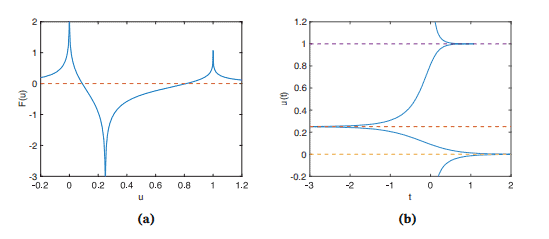
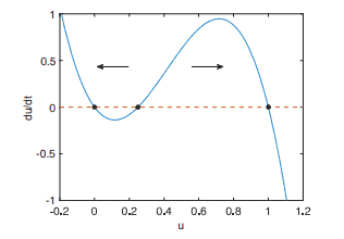
1.2.4. Modeling Chemical Reactions. One of the important uses of differential equations, at least in this book, is to model the dynamics of chemical reactions. The two elementary reactions that are of most importance here are conversion between species, denoted
$$
A \stackrel{\alpha}{\rightleftarrows} B,
$$

called a first order reaction, and formation and degradation of a product from two component species, denoted
$$
A+B \underset{\approx}{\rightleftarrows} C
$$
called a second order reaction.
The differential equations describing the first of these are
$$
\frac{d a}{d t}=\beta b-\alpha a, \quad \frac{d b}{d t}=-\beta b+\alpha a
$$
where $a=[A]$ and $b=[B]$, is the statement in math symbols that $B$ is created from $A$ at rate $\alpha[A]$ and $A$ is created from $B$ at rate $\beta[B]$. Of course, the total of $A$ and $B$ is a conserved quantity, since $\frac{d}{d t}(a+b)=0$.
The second of these reactions is described by the three differential equations
$$
\frac{d a}{d t}=-\gamma a b+\delta c, \quad \frac{d b}{d t}=-\gamma a b+\delta c, \quad \frac{d c}{d t}=\gamma a b-\delta c
$$
where $c=[C]$, which puts into math symbols the fact that $C$ is created from the combination of $A$ and $B$ at a rate that is proportional to the product $[A][B]$, called the law of mass action. Notice that the units of $\gamma$ are different ((time) ${ }^{-1}$ (concentration $)^{-1}$ ) than those for first order reactions ((time) $\left.{ }^{-1}\right)$. The degradation of $C$ into $A$ and $B$ is a first order reaction. For this reaction there are two conserved quantities, namely $[A]+[C]$ and $[B]+[C]$

An important example of reaction kinetics occurs in the study of epidemics, with the so-called SIR epidemic. Here $S$ represents susceptible individuals, I represents infected individuals, and $R$ represents recovered or removed individuals. We represent the disease process by the reaction scheme
$$
S+I \stackrel{\alpha}{\longrightarrow} 2 I, \quad I \stackrel{\beta}{\longrightarrow} R
$$
This implies that a susceptible individual can become infected following contact with an infected individual, and that infected individuals recover at an exponential rate.

数学代写|微分方程代写differential equation代考|Stochastic Processes

1.3.1. Decay Processes. Now that we have the review of differential equations behind us, we must face the fact that differential equation descriptions of biological processes are at best, highly idealized. This is because biological processes, and in fact many physical processes, are not deterministic, but noisy, or stochastic. This noise, or randomness, could be because, while the process actually is deterministic, we do not have the ability or the patience to accurately calculate the outcome of the process. For example, the flipping of a coin or the spin of a roulette wheel has a deterministic result, in that, if initial conditions were known with sufficient accuracy, an accurate calculation of the end result could be made. However, this is so impractical that it is not worth pursuing. Similarly, the motion of water vapor molecules in the air is by completely deterministic process (following Newton’s Second Law, no quantum physics required) but determining the behavior of a gas by solving the governing differential equations for the position of each particle is completely out of the question.

There are other processes for which deterministic laws are not even known. This is because they are governed by quantum dynamics, having possible changes of state that cannot be described by a deterministic equation. For example, the decay of a radioactive particle and the change of conformation of a protein molecule, such as an ion channel, cannot, as far as we know, be described by a deterministic process. Similarly, the mistakes made by the reproductive machinery of a cell when duplicating its DNA (i.e., the mutations) cannot, as far as we currently know, be described by a deterministic process.

Given this reality, we are forced to come up with another way to describe interesting processes. And this is by keeping track of various statistics as time proceeds. For example, it may not be possible to exactly track the numbers of people who get the flu every year, but an understanding of how the average number changes over several years may be sufficient for health care policy makers. Similarly, with carbon dating techniques, it is not necessary to know exactly how many carbon- 14 molecules there are in a particular painting at a particular time, but an estimate of an average or expected number of molecules can be sufficient to decide if the painting is genuine or a forgery.
1.3.1.1. Probability Theory. To make some progress in this way of describing things, we must define some terms. First, there must be some object that we wish to measure or quantify, also called a random variable, and the collection of all possible outcomes of this measurement is called its state space, or sample space. For example, the flip of a coin can result in it landing with head or tail up, and these two outcomes constitute the state space. Similarly, an ion channel may at any given time be either open or closed, and this also constitutes its state space. The random variable could be a discrete or continuous variable taking on only integer values if it is discrete or a real valued number or vector if it is continuous.

数学代写|微分方程代写differential equation代考|Several Reactions

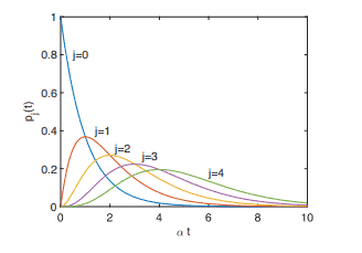
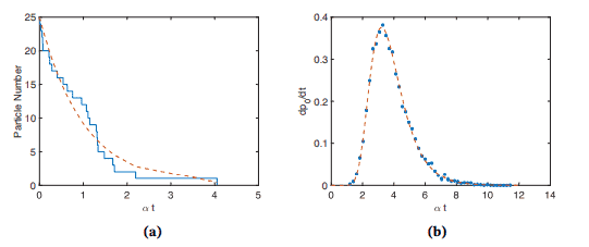
1.3.2. Several Reactions. In the example of particle decay there was only one reaction possible. However, this is not typical as most chemical reactions involve a range of possible reactions. For example, suppose a particle (like a bacterium) may reproduce at some rate or it may die at a different rate. The question addressed here is how to do a stochastic simulation of this process.

Suppose the state $S_{j}$ can transition to the state $S_{k}$ at rate $\lambda_{k j}$. To do a stochastic simulation of this process, we must decide when the next reaction takes place and which reaction it is that takes place.

To decide when the next reaction takes place, we use the fact that the probability that the next reaction has taken place by time $t$ is 1 minus the probability that the next reaction has not taken place by time $t$. Furthermore, the probability that the reaction from state $j$ to state $k$ has not taken place by time $t$ is $\exp \left(-\lambda_{k j} t\right)$. So, the probability that no reaction has taken place by time $t$ (since these reactions are assumed to be independent) is
$$
\prod_{k} \exp \left(-\lambda_{k j} t\right)=\exp \left(-\sum_{k} \lambda_{k j} t\right) .
$$
It follows that the cdf for the next reaction is
$$
1-\exp \left(-\sum_{k} \lambda_{k j} t\right)=1-\exp (-r t),
$$
where $r=\sum_{k} \lambda_{k j}$. In other words, the next reaction is an exponential process with rate $r$
Next, the probability that the next reaction is the $i$ th reaction $S_{j} \rightarrow S_{i}$ is
$$
p_{i j}=\frac{\lambda_{i j}}{\sum_{k} \lambda_{k j}}=\frac{\lambda_{i j}}{r} .
$$
To be convinced of this, apply the results of Exercise $1.26$ to the case where either the $S_{j} \rightarrow S_{i}$ reaction occurs first or another reaction occurs first.

With these facts in hand, as we did above, we pick the next reaction time increment to be
$$
\dot{\delta} t=\frac{-1}{r} \ln R_{1} \text {, }
$$
where $0<R_{1}<1$ is a uniformly distributed random number. Next, to decide which of the reactions to implement, construct the vector $x_{k}=\frac{1}{r} \sum_{i=1}^{k} \lambda_{i j}$, the scaled vector of cumulative sums of $\lambda_{i j}$. Notice that the vector $x_{k}$ is ordered with $0 \leq x_{1} \leq x_{2} \leq \cdots \leq$ $x_{N}=1$, where $N$ is the total number of states. Now, pick a second random number $R_{2}$, uniformly distributed between zero and one, and pick the next reaction to be $S_{j} \rightarrow S_{k}$ where
$$
k=\min {j}\left{R{2} \leq x_{j}\right}
$$

微分方程代考

数学代写|微分方程代写differential equation代考|Modeling Chemical Reactions

1.2.4。模拟化学反应。至少在本书中，微分方程的重要用途之一是模拟化学反应的动力学。这里最重要的两个基本反应是物种之间的转化，表示为

一个⇄一个乙,

称为一级反应，以及由两种组分物质形成和降解产物，表示为

一个+乙⇄≈C
称为二级反应。
描述第一个的微分方程是

d一个d吨=bb−一个一个,dbd吨=−bb+一个一个
在哪里一个=[一个]和b=[乙], 是数学符号中的陈述乙创建自一个以速率一个[一个]和一个创建自乙以速率b[乙]. 当然，总一个和乙是一个守恒量，因为dd吨(一个+b)=0.
这些反应中的第二个由三个微分方程描述

d一个d吨=−C一个b+dC,dbd吨=−C一个b+dC,dCd吨=C一个b−dC
在哪里C=[C]，这将以下事实放入数学符号中C是从组合创建的一个和乙以与产品成比例的速率[一个][乙]，称为质量作用定律。请注意，单位C不同（（时间）−1（专注)−1) 比一级反应 ((time)−1). 的退化C进入一个和乙是一级反应。对于这个反应有两个守恒量，即[一个]+[C]和[乙]+[C]

反应动力学的一个重要例子发生在流行病的研究中，即所谓的 SIR 流行病。这里小号代表易感个体，I 代表受感染个体，并且R代表恢复或移除的个人。我们用反应方案来表示疾病过程

小号+我⟶一个2我,我⟶bR
这意味着易感个体在与受感染个体接触后可能会被感染，并且受感染个体会以指数速度恢复。

数学代写|微分方程代写differential equation代考|Stochastic Processes

1.3.1。衰减过程。既然我们已经回顾了微分方程，我们必须面对这样一个事实，即生物过程的微分方程描述充其量是高度理想化的。这是因为生物过程，实际上是许多物理过程，不是确定性的，而是嘈杂的或随机的。这种噪音或随机性可能是因为虽然过程实际上是确定性的，但我们没有能力或耐心来准确计算过程的结果。例如，掷硬币或转动轮盘赌具有确定性结果，因为如果初始条件足够准确，则可以对最终结果进行准确计算。然而，这太不切实际了，不值得追求。相似地，

还有其他一些过程甚至不知道确定性定律。这是因为它们受量子动力学控制，可能会发生无法用确定性方程描述的状态变化。例如，就我们所知，放射性粒子的衰变和蛋白质分子（如离子通道）的构象变化不能用确定性过程来描述。同样，就我们目前所知，细胞的生殖机制在复制其 DNA（即突变）时所犯的错误不能用确定性过程来描述。

鉴于这一现实，我们不得不想出另一种方式来描述有趣的过程。这是通过随着时间的推移跟踪各种统计数据。例如，可能无法准确跟踪每年感染流感的人数，但了解平均人数在几年内的变化可能对医疗保健政策制定者来说就足够了。类似地，使用碳测年技术，不必确切知道特定绘画中在特定时间有多少碳 14 分子，但对平均或预期分子数量的估计就足以决定绘画是否是真品还是赝品。
1.3.1.1。概率论。为了在这种描述事物的方式上取得一些进展，我们必须定义一些术语。首先，必须有一些我们希望测量或量化的对象，也称为随机变量，并且该测量的所有可能结果的集合称为其状态空间或样本空间。例如，抛硬币会导致它头朝上或尾部朝上落地，这两种结果构成了状态空间。类似地，离子通道可以在任何给定时间打开或关闭，这也构成了它的状态空间。随机变量可以是离散变量或连续变量，如果它是离散的，则它可以是仅取整数值的变量，或者如果它是连续的，则可以是实数值或向量。

数学代写|微分方程代写differential equation代考|Several Reactions

1.3.2. 几个反应。在粒子衰变的例子中，只有一种反应可能。然而，这并不典型，因为大多数化学反应都涉及一系列可能的反应。例如，假设一个粒子（如细菌）可能以某种速度繁殖，或者它可能以不同的速度死亡。这里解决的问题是如何对这个过程进行随机模拟。

假设状态小号j可以过渡到状态小号ķ以速率λķj. 要对这个过程进行随机模拟，我们必须确定下一个反应何时发生以及发生的是哪个反应。

为了确定下一个反应何时发生，我们使用了下一个反应发生的概率按时间计算的事实吨是 1 减去按时间没有发生下一个反应的概率吨. 此外，来自状态的反应的概率j陈述ķ没有按时发生吨是经验⁡(−λķj吨). 因此，按时间没有发生反应的概率吨（因为假设这些反应是独立的）是

∏ķ经验⁡(−λķj吨)=经验⁡(−∑ķλķj吨).
因此，下一个反应的 cdf 是

1−经验⁡(−∑ķλķj吨)=1−经验⁡(−r吨),
在哪里r=∑ķλķj. 换句话说，下一个反应是一个指数过程，速率r
接下来，下一个反应的概率是一世反应小号j→小号一世是

p一世j=λ一世j∑ķλķj=λ一世jr.
要确信这一点，请应用练习的结果1.26的情况下，无论是小号j→小号一世反应先发生或另一个反应先发生。

有了这些事实，正如我们上面所做的那样，我们选择下一个反应时间增量为

d˙吨=−1rln⁡R1, 
在哪里0<R1<1是一个均匀分布的随机数。接下来，要决定执行哪些反应，请构建向量Xķ=1r∑一世=1ķλ一世j, 的累积和的缩放向量λ一世j. 注意向量Xķ订购0≤X1≤X2≤⋯≤ Xñ=1， 在哪里ñ是状态的总数。现在，选择第二个随机数R2, 均匀分布在 0 和 1 之间，并选择下一个反应为小号j→小号ķ在哪里

k=\min {j}\left{R{2} \leq x_{j}\right}

统计代写请认准statistics-lab™. statistics-lab™为您的留学生涯保驾护航。

金融工程代写

金融工程是使用数学技术来解决金融问题。金融工程使用计算机科学、统计学、经济学和应用数学领域的工具和知识来解决当前的金融问题，以及设计新的和创新的金融产品。

非参数统计代写

非参数统计指的是一种统计方法，其中不假设数据来自于由少数参数决定的规定模型；这种模型的例子包括正态分布模型和线性回归模型。

广义线性模型代考

广义线性模型（GLM）归属统计学领域，是一种应用灵活的线性回归模型。该模型允许因变量的偏差分布有除了正态分布之外的其它分布。

术语 广义线性模型（GLM）通常是指给定连续和/或分类预测因素的连续响应变量的常规线性回归模型。它包括多元线性回归，以及方差分析和方差分析（仅含固定效应）。

有限元方法代写

有限元方法（FEM）是一种流行的方法，用于数值解决工程和数学建模中出现的微分方程。典型的问题领域包括结构分析、传热、流体流动、质量运输和电磁势等传统领域。

有限元是一种通用的数值方法，用于解决两个或三个空间变量的偏微分方程（即一些边界值问题）。为了解决一个问题，有限元将一个大系统细分为更小、更简单的部分，称为有限元。这是通过在空间维度上的特定空间离散化来实现的，它是通过构建对象的网格来实现的：用于求解的数值域，它有有限数量的点。边界值问题的有限元方法表述最终导致一个代数方程组。该方法在域上对未知函数进行逼近。[1] 然后将模拟这些有限元的简单方程组合成一个更大的方程系统，以模拟整个问题。然后，有限元通过变化微积分使相关的误差函数最小化来逼近一个解决方案。

tatistics-lab作为专业的留学生服务机构，多年来已为美国、英国、加拿大、澳洲等留学热门地的学生提供专业的学术服务，包括但不限于Essay代写，Assignment代写，Dissertation代写，Report代写，小组作业代写，Proposal代写，Paper代写，Presentation代写，计算机作业代写，论文修改和润色，网课代做，exam代考等等。写作范围涵盖高中，本科，研究生等海外留学全阶段，辐射金融，经济学，会计学，审计学，管理学等全球99%专业科目。写作团队既有专业英语母语作者，也有海外名校硕博留学生，每位写作老师都拥有过硬的语言能力，专业的学科背景和学术写作经验。我们承诺100%原创，100%专业，100%准时，100%满意。

随机分析代写

随机微积分是数学的一个分支，对随机过程进行操作。它允许为随机过程的积分定义一个关于随机过程的一致的积分理论。这个领域是由日本数学家伊藤清在第二次世界大战期间创建并开始的。

时间序列分析代写

随机过程，是依赖于参数的一组随机变量的全体，参数通常是时间。 随机变量是随机现象的数量表现，其时间序列是一组按照时间发生先后顺序进行排列的数据点序列。通常一组时间序列的时间间隔为一恒定值（如1秒，5分钟，12小时，7天，1年），因此时间序列可以作为离散时间数据进行分析处理。研究时间序列数据的意义在于现实中，往往需要研究某个事物其随时间发展变化的规律。这就需要通过研究该事物过去发展的历史记录，以得到其自身发展的规律。

回归分析代写

多元回归分析渐进（Multiple Regression Analysis Asymptotics）属于计量经济学领域，主要是一种数学上的统计分析方法，可以分析复杂情况下各影响因素的数学关系，在自然科学、社会和经济学等多个领域内应用广泛。

MATLAB代写

MATLAB 是一种用于技术计算的高性能语言。它将计算、可视化和编程集成在一个易于使用的环境中，其中问题和解决方案以熟悉的数学符号表示。典型用途包括：数学和计算算法开发建模、仿真和原型制作数据分析、探索和可视化科学和工程图形应用程序开发，包括图形用户界面构建MATLAB 是一个交互式系统，其基本数据元素是一个不需要维度的数组。这使您可以解决许多技术计算问题，尤其是那些具有矩阵和向量公式的问题，而只需用 C 或 Fortran 等标量非交互式语言编写程序所需的时间的一小部分。MATLAB 名称代表矩阵实验室。MATLAB 最初的编写目的是提供对由 LINPACK 和 EISPACK 项目开发的矩阵软件的轻松访问，这两个项目共同代表了矩阵计算软件的最新技术。MATLAB 经过多年的发展，得到了许多用户的投入。在大学环境中，它是数学、工程和科学入门和高级课程的标准教学工具。在工业领域，MATLAB 是高效研究、开发和分析的首选工具。MATLAB 具有一系列称为工具箱的特定于应用程序的解决方案。对于大多数 MATLAB 用户来说非常重要，工具箱允许您学习和应用专业技术。工具箱是 MATLAB 函数（M 文件）的综合集合，可扩展 MATLAB 环境以解决特定类别的问题。可用工具箱的领域包括信号处理、控制系统、神经网络、模糊逻辑、小波、仿真等。

R语言代写	问卷设计与分析代写
PYTHON代写	回归分析与线性模型代写
MATLAB代写	方差分析与试验设计代写
STATA代写	机器学习/统计学习代写
SPSS代写	计量经济学代写
EVIEWS代写	时间序列分析代写
EXCEL代写	深度学习代写
SQL代写	各种数据建模与可视化代写

如果你也在 怎样代写微分方程differential equation这个学科遇到相关的难题，请随时右上角联系我们的24/7代写客服。

微分方程（ODE）是一个微分方程，包含一个或多个独立变量的函数以及这些函数的导数。术语普通是与术语偏微分方程相对应的，后者可能与一个以上的独立变量有关。

statistics-lab™ 为您的留学生涯保驾护航 在代写微分方程differential equation方面已经树立了自己的口碑, 保证靠谱, 高质且原创的统计Statistics代写服务。我们的专家在代写微分方程differential equation代写方面经验极为丰富，各种代写微分方程differential equation相关的作业也就用不着说。

我们提供的微分方程differential equation及其相关学科的代写，服务范围广, 其中包括但不限于:

• Statistical Inference 统计推断
• Statistical Computing 统计计算
• Advanced Probability Theory 高等概率论
• Advanced Mathematical Statistics 高等数理统计学
• (Generalized) Linear Models 广义线性模型
• Statistical Machine Learning 统计机器学习
• Longitudinal Data Analysis 纵向数据分析
• Foundations of Data Science 数据科学基础

数学代写|微分方程代写differential equation代考|Background Material

1.1.1. Partial Derivatives. In what is to come, we will be dealing with functions of both space and time. We may be interested in the electrolyte balance within muscle tissue, or the distribution of microorganisms occupying a lake; either way, we are studying how something occupying a region in space evolves over time. We often describe position in this space by using the Cartesian coordinates $x, y$, and $z$, and time by the variable $t$ (although other coordinate representations like polar or spherical coordinates are sometimes useful).

The quantity of interest may be the concentration (= number per unit volume) of calcium ions in a cell or the concentration of microorganisms in the lake, but it is typically denoted by some scalar function $u=u(x, y, z, t)$. If $u$ changes smoothly in time, then it has a time derivative $\frac{\partial u}{\partial t}$ defined by ${ }^{1}$
$$
\frac{\partial u}{\partial t}=\lim {\Delta t \rightarrow 0} \frac{u(x, y, z, t+\Delta t)-u(x, y, z, t)}{\Delta t} $$ The fundamental theorem of calculus states that $$ u(x, y, z, b)-u(x, y, z, a)=\int{a}^{b} \frac{\partial u}{\partial t} d t
$$
In words, the cumulative change in $u$ over an interval of time can be measured by observing the difference between $u$ at the end and the beginning of the interval.

Similarly, if $u$ varies smoothly in space, spatial derivatives can be defined, such as
$$
\frac{\partial u}{\partial x}=\lim _{\Delta x \rightarrow 0} \frac{u(x+\Delta x, y, z, t)-u(x, y, z, t)}{\Delta x},
$$
and this is one component of the gradient of $u$, the vector-valued function
$$
\nabla u=\left(\frac{\partial u}{\partial x}, \frac{\partial u}{\partial y}, \frac{\partial u}{\partial z}\right)
$$
The gradient holds all of the information we need about how $u$ changes in space, but since there are an infinite number of directions in which we could move from a particular point, to find the derivative of $u$ in a particular direction, $\mathbf{v}$, where $\mathbf{v}$ is a unit vector, we define the directional derivative,
$$
\frac{\partial u}{\partial \mathbf{v}}=\nabla u \cdot \mathbf{v} \text {. }
$$
One important object that uses the gradient is
$$
\mathbf{n}=\frac{\nabla u}{|\nabla u|},
$$
which, provided $|\nabla u| \neq 0$, is a unit vector pointing in the direction of the greatest increase of the function $u$. The importance of this to a skier or snowboarder is obvious, pointing in the direction parallel to the “fall-line”. It is also noteworthy that $\mathbf{n}$ is perpendicular (orthogonal) to level surfaces of the function $u$. We can verify this by noting that if $(x(s), y(s), z(s))$ is a curve in space parametrized by $s$, the tangent direction of the curve is the vector $(\dot{x}(s), \dot{y}(s), \dot{z}(s))$. If the function $u(x, y, z)$ is a constant on this curve, $u(x(s), y(s), z(s))=C$, then differentiating this with respect to $s$, we find that
$$
0=\frac{\partial u}{\partial x} \dot{x}(s)+\frac{\partial u}{\partial y} \dot{y}(s)+\frac{\partial u}{\partial z} \approx(s) \equiv \nabla u \cdot\left(\begin{array}{c}
\dot{x}(s) \
\dot{y}(s) \
\dot{z}(s)
\end{array}\right)
$$
as claimed.

数学代写|微分方程代写differential equation代考|Ordinary Differential Equations

1.2.1. First Order Equations. An nrdinary differential equation specifies a relationship between the (time) derivative of some quantity $u$ and its values through, say,
$$
\frac{d u}{d t}=f(u, t) .
$$
This equation is autonomous if $f$ is independent of $t$, so that
$$
\frac{d u}{d t}=f(u) .
$$
Many of the problems discussed in this book are autonomous in time.
If $u$ is a scalar quantity, the solution of equation (1.25) can be readily understood using graphical means, i.e., by plotting $\frac{d u}{d t}$ vs. $u$. An example is shown in Figure $1.1$.
Figure 1.1. Plot of $\frac{d u}{d t}$ vs. $u$ for the bistable function $f(u)=a u(1-u)(u-\alpha)$ with $\alpha=0.25, a=10 .$
The first things to notice are the zeros of $f(u)$, i.e., the equilibria. For the example $f(u)=a u(u-1)(\alpha-u)$, shown in Figure 1.1, the equilibria are at $u_{0}=0, u_{0}=$ $\alpha$, and $u_{0}=1$. Next, one can determine the direction of movement if $u$ is not at an equilibrium. These are shown with arrows in Figure 1.1. For example, if $00$ so that $u$ is increasing there. This is our first indication that $u_{0}=0$ and $u_{0}=1$ are stable equilibria, while $u_{0}=\alpha$ is unstable.

The next thing to do is to linearize the equations about the equilibria. Linearization is a very important procedure by which one reduces a nonlinear equation to a linear equation. ${ }^{3}$ It is a good idea to understand it thoroughly, because it is used often in this text.

数学代写|微分方程代写differential equation代考|Systems of first order equations

1.2.2. Systems of first order equations. We now turn our attention to systems of first order equations, which can still be written in the form of (1.24) provided we recognize that $u$ is a vector, rather than a scalar, quantity. The most important example for this text is when there are two unknown scalar functions $u(t)$ and $v(t)$ and the equations describing their evolution are in the form
$$
\begin{aligned}
\frac{d u}{d t} &=f(u, v) \
\frac{d v}{d t} &=g(u, v)
\end{aligned}
$$
As with first order equations, a useful way to proceed is with a graphical, or phase plane, analysis. The first step of this analysis is to plot the nullclines, the curves in the $u-v$ plane along which either $u$ or $v$ do not change, i.e., $\frac{d u}{d t}=0$ or $\frac{d v}{d t}=0$.

There are many examples of this procedure in this book, however, for purposes of illustration, let’s look at solutions of the second order differential equation
$$
\frac{d^{2} u}{d t^{2}}+f(u)=0
$$
where $f(u)=a u(1-u)(u-\alpha)$, the same function as used above. To write this equation as a first order system, we set $v=\frac{d u}{d t}$, and then the equations are
$$
\begin{aligned}
&\frac{d u}{d t}=v \
&\frac{d v}{d t}=-f(u)
\end{aligned}
$$
The nullclines for this system are easily determined, being the line $v=0$ for the $u$ nullcline, and $f(u)=0$ for the $v$ nullclines, i.e., the lines $u=0, u=\alpha$, and $u=1$. These are shown plotted in Figure $1.3$ as dashed lines.

The next step is to identify all the critical points, i.e., the points at which $\frac{d u}{d t}$ and $\frac{d v}{d t}$ are simultaneously zero, hence, points of equilibrium. These are, of course, all the intersections of the $u$ and $v$ nullclines. For this example, they are the points with $v=0$ and $u=0, \alpha$ and 1 .

微分方程代考

数学代写|微分方程代写differential equation代考|Background Material

1.1.1。偏导数。在接下来的内容中，我们将处理空间和时间的功能。我们可能对肌肉组织内的电解质平衡或占据湖泊的微生物分布感兴趣；无论哪种方式，我们都在研究占据空间区域的事物如何随着时间的推移而演变。我们经常使用笛卡尔坐标来描述这个空间中的位置X,是， 和和, 和时间由变量吨（尽管有时极坐标或球坐标等其他坐标表示很有用）。

感兴趣的量可能是细胞中钙离子的浓度（=每单位体积的数量）或湖中微生物的浓度，但它通常由一些标量函数表示在=在(X,是,和,吨). 如果在随时间平滑变化，则有时间导数∂在∂吨被定义为1

∂在∂吨=林Δ吨→0在(X,是,和,吨+Δ吨)−在(X,是,和,吨)Δ吨微积分基本定理指出

在(X,是,和,b)−在(X,是,和,一个)=∫一个b∂在∂吨d吨
换句话说，累积变化在可以通过观察一段时间内的差异来测量在在间隔的结束和开始。

同样，如果在在空间上平滑变化，可以定义空间导数，例如

∂在∂X=林ΔX→0在(X+ΔX,是,和,吨)−在(X,是,和,吨)ΔX,
这是梯度的一个组成部分在, 向量值函数

∇在=(∂在∂X,∂在∂是,∂在∂和)
梯度包含我们需要的所有信息在空间的变化，但是由于我们可以从一个特定点移动的方向有无数个，因此要找到在在特定的方向，在， 在哪里在是单位向量，我们定义方向导数，

∂在∂在=∇在⋅在. 
使用渐变的一个重要对象是

n=∇在|∇在|,
其中，提供|∇在|≠0, 是指向函数最大增量方向的单位向量在. 这对滑雪者或单板滑雪者的重要性是显而易见的，指向与“下降线”平行的方向。还值得注意的是n与函数的水平面垂直（正交）在. 我们可以通过注意到如果(X(s),是(s),和(s))是一条空间曲线，参数化为s，曲线的切线方向为向量(X˙(s),是˙(s),和˙(s)). 如果函数在(X,是,和)在这条曲线上是一个常数，在(X(s),是(s),和(s))=C，然后将其区分为s, 我们发现

0=∂在∂XX˙(s)+∂在∂是是˙(s)+∂在∂和≈(s)≡∇在⋅(X˙(s) 是˙(s) 和˙(s))
如声称的那样。

数学代写|微分方程代写differential equation代考|Ordinary Differential Equations

1.2.1。一阶方程。一个普通微分方程指定了某个量的（时间）导数之间的关系在以及它的价值，比如说，

d在d吨=F(在,吨).
这个方程是自治的，如果F独立于吨， 以便

d在d吨=F(在).
本书中讨论的许多问题在时间上都是自主的。
如果在是一个标量，方程（1.25）的解可以很容易地使用图形方法来理解，即通过绘制d在d吨对比在. 一个例子如图所示1.1.
图 1.1。情节d在d吨对比在对于双稳态函数F(在)=一个在(1−在)(在−一个)和一个=0.25,一个=10.
首先要注意的是零F(在)，即均衡。例如F(在)=一个在(在−1)(一个−在)，如图 1.1 所示，平衡点位于在0=0,在0= 一个， 和在0=1. 接下来，可以确定运动的方向，如果在不处于平衡状态。这些在图 1.1 中用箭头表示。例如，如果00以便在那里正在增加。这是我们的第一个迹象表明在0=0和在0=1是稳定的平衡，而在0=一个不稳定。

接下来要做的是线性化关于平衡的方程。线性化是一个非常重要的过程，通过它可以将非线性方程简化为线性方程。3彻底理解它是个好主意，因为它在本文中经常使用。

数学代写|微分方程代写differential equation代考|Systems of first order equations

1.2.2。一阶方程组。我们现在将注意力转向一阶方程组，只要我们认识到在是一个向量，而不是一个标量，数量。本文最重要的例子是当有两个未知的标量函数时在(吨)和在(吨)描述它们演化的方程是

d在d吨=F(在,在) d在d吨=G(在,在)
与一阶方程一样，一种有用的方法是使用图形或相平面分析。该分析的第一步是绘制零斜线，即在−在沿哪个平面在或者在不要改变，即d在d吨=0或者d在d吨=0.

本书中有很多这个过程的例子，然而，为了说明的目的，让我们看看二阶微分方程的解

d2在d吨2+F(在)=0
在哪里F(在)=一个在(1−在)(在−一个)，与上面使用的功能相同。为了把这个方程写成一阶系统，我们设置在=d在d吨，然后方程是

d在d吨=在 d在d吨=−F(在)
该系统的零斜线很容易确定，即在=0为了在零斜线，和F(在)=0为了在nullclines，即线条在=0,在=一个， 和在=1. 这些显示在图1.3作为虚线。

下一步是识别所有关键点，即d在d吨和d在d吨同时为零，因此是平衡点。当然，这些都是在和在空斜线。对于这个例子，它们是与在=0和在=0,一个和 1。

统计代写请认准statistics-lab™. statistics-lab™为您的留学生涯保驾护航。

金融工程代写

金融工程是使用数学技术来解决金融问题。金融工程使用计算机科学、统计学、经济学和应用数学领域的工具和知识来解决当前的金融问题，以及设计新的和创新的金融产品。

非参数统计代写

非参数统计指的是一种统计方法，其中不假设数据来自于由少数参数决定的规定模型；这种模型的例子包括正态分布模型和线性回归模型。

广义线性模型代考

广义线性模型（GLM）归属统计学领域，是一种应用灵活的线性回归模型。该模型允许因变量的偏差分布有除了正态分布之外的其它分布。

术语 广义线性模型（GLM）通常是指给定连续和/或分类预测因素的连续响应变量的常规线性回归模型。它包括多元线性回归，以及方差分析和方差分析（仅含固定效应）。

有限元方法代写

有限元方法（FEM）是一种流行的方法，用于数值解决工程和数学建模中出现的微分方程。典型的问题领域包括结构分析、传热、流体流动、质量运输和电磁势等传统领域。

有限元是一种通用的数值方法，用于解决两个或三个空间变量的偏微分方程（即一些边界值问题）。为了解决一个问题，有限元将一个大系统细分为更小、更简单的部分，称为有限元。这是通过在空间维度上的特定空间离散化来实现的，它是通过构建对象的网格来实现的：用于求解的数值域，它有有限数量的点。边界值问题的有限元方法表述最终导致一个代数方程组。该方法在域上对未知函数进行逼近。[1] 然后将模拟这些有限元的简单方程组合成一个更大的方程系统，以模拟整个问题。然后，有限元通过变化微积分使相关的误差函数最小化来逼近一个解决方案。

tatistics-lab作为专业的留学生服务机构，多年来已为美国、英国、加拿大、澳洲等留学热门地的学生提供专业的学术服务，包括但不限于Essay代写，Assignment代写，Dissertation代写，Report代写，小组作业代写，Proposal代写，Paper代写，Presentation代写，计算机作业代写，论文修改和润色，网课代做，exam代考等等。写作范围涵盖高中，本科，研究生等海外留学全阶段，辐射金融，经济学，会计学，审计学，管理学等全球99%专业科目。写作团队既有专业英语母语作者，也有海外名校硕博留学生，每位写作老师都拥有过硬的语言能力，专业的学科背景和学术写作经验。我们承诺100%原创，100%专业，100%准时，100%满意。

随机分析代写

随机微积分是数学的一个分支，对随机过程进行操作。它允许为随机过程的积分定义一个关于随机过程的一致的积分理论。这个领域是由日本数学家伊藤清在第二次世界大战期间创建并开始的。

时间序列分析代写

随机过程，是依赖于参数的一组随机变量的全体，参数通常是时间。 随机变量是随机现象的数量表现，其时间序列是一组按照时间发生先后顺序进行排列的数据点序列。通常一组时间序列的时间间隔为一恒定值（如1秒，5分钟，12小时，7天，1年），因此时间序列可以作为离散时间数据进行分析处理。研究时间序列数据的意义在于现实中，往往需要研究某个事物其随时间发展变化的规律。这就需要通过研究该事物过去发展的历史记录，以得到其自身发展的规律。

回归分析代写

多元回归分析渐进（Multiple Regression Analysis Asymptotics）属于计量经济学领域，主要是一种数学上的统计分析方法，可以分析复杂情况下各影响因素的数学关系，在自然科学、社会和经济学等多个领域内应用广泛。

MATLAB代写

MATLAB 是一种用于技术计算的高性能语言。它将计算、可视化和编程集成在一个易于使用的环境中，其中问题和解决方案以熟悉的数学符号表示。典型用途包括：数学和计算算法开发建模、仿真和原型制作数据分析、探索和可视化科学和工程图形应用程序开发，包括图形用户界面构建MATLAB 是一个交互式系统，其基本数据元素是一个不需要维度的数组。这使您可以解决许多技术计算问题，尤其是那些具有矩阵和向量公式的问题，而只需用 C 或 Fortran 等标量非交互式语言编写程序所需的时间的一小部分。MATLAB 名称代表矩阵实验室。MATLAB 最初的编写目的是提供对由 LINPACK 和 EISPACK 项目开发的矩阵软件的轻松访问，这两个项目共同代表了矩阵计算软件的最新技术。MATLAB 经过多年的发展，得到了许多用户的投入。在大学环境中，它是数学、工程和科学入门和高级课程的标准教学工具。在工业领域，MATLAB 是高效研究、开发和分析的首选工具。MATLAB 具有一系列称为工具箱的特定于应用程序的解决方案。对于大多数 MATLAB 用户来说非常重要，工具箱允许您学习和应用专业技术。工具箱是 MATLAB 函数（M 文件）的综合集合，可扩展 MATLAB 环境以解决特定类别的问题。可用工具箱的领域包括信号处理、控制系统、神经网络、模糊逻辑、小波、仿真等。

R语言代写	问卷设计与分析代写
PYTHON代写	回归分析与线性模型代写
MATLAB代写	方差分析与试验设计代写
STATA代写	机器学习/统计学习代写
SPSS代写	计量经济学代写
EVIEWS代写	时间序列分析代写
EXCEL代写	深度学习代写
SQL代写	各种数据建模与可视化代写